Four-Vectors (4-Vectors) & Lorentz Invariants of Special Relativity:
A Study of Elegant Physics
The Ultimate
Four-Vector & Lorentz Invariant Reference
The Four-Vectors (4-Vectors) and Lorentz Invariants of Special
Relativistic (SR) theory are fundamental entities that accurately,
precisely, and beautifully describe the physical properties of the world
around us. While it is known that SR is not the "deepest" theory, it is
valid for the majority of the known universe. It is believed to apply to
all forms of interaction, including that of fundamental particles and
quantum effects, with the only exception being that of large-scale
gravitational phenomena, where spacetime itself is significantly curved,
for which General Relativity (GR) is required. The SR 4-vector notation is
one of the most powerful tools in understanding the physics of the
universe, as it simplifies a great many of the physical relations.
Welcome to Relativistic Quantum Reality: Virtual worlds of imaginary particles: The dreams stuff is made of: Life, the eternal ghost in the machine...
This site is dedicated to the quest for knowledge and wisdom, through science, mathematics, philosophy, invention, and technology. May the treasures buried herein spark the fires of imagination like the twinkling jewels of celestial light crowning the midnight sky...
A vector is a mathematical object which has both magnitude and direction.
It is a powerful tool for describing physical phenomena. A common 3-vector
is the velocity vector (vx, vy, vz),
which tells you in what direction and how fast something is moving.
One might use the (x, y, z) coordinates to write down the velocity vector
of some object in the laboratory. That would be an example of a
rectilinear coordinate system. Another person might use a coordinate
system that is rotated wrt. the first observer, with components (y', x',
z). The same vector might also be described by the (r, θ, φ) spherical
coordinate system. Within a given coordinate system, each component is
typically orthogonal to each other component. While these different
coordinate systems will usually have different numbers in the vector
3-tuple, they nevertheless describe the same vector and the same physics.
Hence, the vector can be considered the "primary" element, which is then
described by any number of different coordinate systems, which simply
represent one point-of-view of the given vector.
The extension of 3-vectors to that of 4-vectors is a simple idea. Let's
imagine some <event> in spacetime. The location of the <event> in the
Newtonian world would be it's 3-position (x,y,z), and the time (t) at
which it occurs. In the Newtonian world these are totally separate ideas.
SR unites them into a single object. The location of the <event> in the SR
world would be it's 4-position (ct,x,y,z). All that we have done is to
insert the time (t) into the vector as another component. The factor of
(c) is put with it to make the dimensional units work out right. (
[m/s]*[s] = [m]). So, each component now has overall units of [m] for this
4-vector. This rather simple idea, combined with the postulates of SR,
lead to some amazing results and elegant simplifications of physical
concepts...
There are two postulates which lead to all of SR-Special Relativity: (1) The laws of physics are the same for all inertial reference frames.
This means the form of the physical laws should not change for different
inertial observers. This can be also restated as "All inertial observers
measure the same interval magnitude between two <event>'s". I say it this way
because all of experimental physics ultimately boils down to taking a
measurement. Yet another way to say it is that the result of any Poincaré Transformation (includes Lorentz Transformations) leaves the Invariant Interval unchanged. (2) The speed of light (c) in vacuum is the same for all inertial
reference frames. This is the result of millions of independent
measurements, all confirming the same observation. This differentiates SR from classical Galilean invariance, which also obeys the first postulate.
4-vectors are tensorial entities which display Poincaré Invariance,
meaning they leave invariant the differential squared interval (ds)2
= (cdt)2-dx2-dy2-dz2. A
consequence of this invariant measurement is that any physical equation
which is written in Poincaré Invariant form is automatically valid for
any inertial reference frame, regardless of how coordinate systems are
arranged. Transformations which leave these vectors unchanged include
fixed translations through space and/or time, rotations through space, and
boosts (coordinate systems moving with constant velocity) through
spacetime. Since 4-vectors are tensors, and Poincaré Invariant, they can
be used to describe and explain the physical properties that are observed
in nature. Although the vector components may change from one reference
frame to another, the 4-vector itself is an invariant, meaning that it
gives valid physical information for all inertial observers. Likewise, the
scalar products of Lorentz Invariant 4-vectors are themselves invariant
quantities, known as Lorentz Scalars. Lorentz Invariance is a
subset of the more general Poincaré Invariance.
The reason that I really like 4-vectors and their notation is that they beautifully and
elegantly display the relations between lots of different physical
properties. They also devolve very nicely into the limiting/approximate
Newtonian cases of {|v|<<c} by letting {γ →1 and dγ/dt →0}. SR
tells us that several different physical properties are actually dual
aspects of the same thing, with the only real difference being one's point
of view, or reference frame. Examples include: (Time , Space), (Energy ,
Momentum), (Power , Force), (Frequency , WaveNumber), (ChargeDensity ,
CurrentDensity), (EM-ScalarPotential , EM-VectorPotential), (Time Differential,
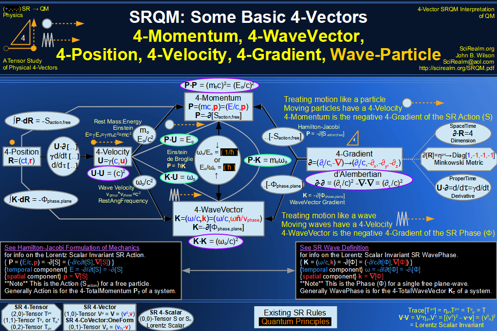
Spatial Gradient), etc. Also, things are even more related than that. The
4-Momentum is just a constant times 4-Velocity. The 4-WaveVector is just a
constant times 4-Momentum. In addition, the very important
conservation/continuity equations seem to just fall out of the notation.
The universe apparently has some simple laws which can be easy to write
down by using a little math and a super notation.
Abbreviations
QM = Quantum Mechanics SR = Special Relativity
SM = Statistical Mechanics GR = General Relativity
Units of Measure - (SI variant, mksC)
length/time
[m] meter <*> [s] second
Count of the quantity of separation or distance; Location of <event>'s in spacetime
mass
[kg] kilogram
Count of the quantity of matter; (the "stuff" at an <event>)
EMcharge
[C] Coulomb
Count of the quantity of electric charge; the Coulomb is more
fundamental than the Ampere
Amperes are just moving Coulombs
temperature
[ºK] Kelvin
Count of the quantity of heat (statistical)
Useful SR Quantities
Velocity vgroup or v or u: v
= cβ = c2/vp = group velocity = <event> velocity= [0..c], {u is historically used in SR
notation} vphase or vp: vp = c/β = c2/v = phase velocity = celerity
= [c..Infinity]
Dimensionless SR Factors:
β = (v/c) = (vgroup/c) = (c/vphase)=
[0..1]: Relativistic Beta factor, the fraction of the speed of light c β = (u/c): Vector form of Beta factor, u is the velocity
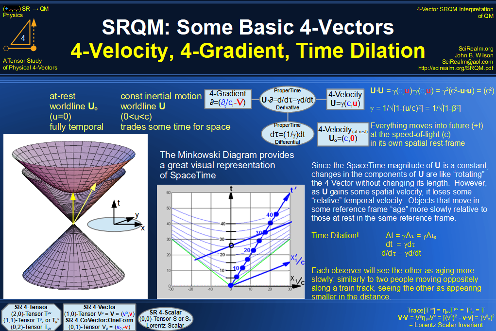
γ[u] = dt/dτ: Lorentz Gamma Scaling Factor (Relativistic Gamma factor)
γ = (1 / √[1-(v/c)2] ) = (1 / √[1-(u·u/c2)]
): Lorentz Gamma Scaling Factor (~1 for v<<c), (>>1 for v~c)
γ = (1 / √[1-β2] ) = (1 / √[1-β·β] ): Lorentz Gamma
Scaling Factor (~1 for β<<1), (>>1 for β~1)
γ = (1 / √[1-β2] ) = 1/√[(1+|β|)/(1-|β|)] : Useful for Doppler Shift Eqns
φ = Ln[γ(1+ β)] ~ Atanh[β]: BoostParameter/Rapidity (which remains
additive in SR, unlike v)
eφ = γ(1+β) = √[(1+β)/(1-β)]
β = Tanh[φ], γ = Cosh[φ], γβ = Sinh[φ], φ = Rapidity (which remains
strictly additive in SR, unlike v)
D = 1 / [γ(1 - β Cos[θ] )] = 1 / [γ(1 - β·n )]: Relativistic
Doppler Factor (sometimes called a relativistic beaming factor)
D+ = γ(1 + β Cos[θ] ): Forward jet Doppler shift
D- = γ(1 - β Cos[θ] ): Counter-jet Doppler shift
Temporal Factors:
τ = t / γ : Proper Time = Rest Time (time as measured in a frame at rest)
dτ = dt / γ : Differential of Proper Time
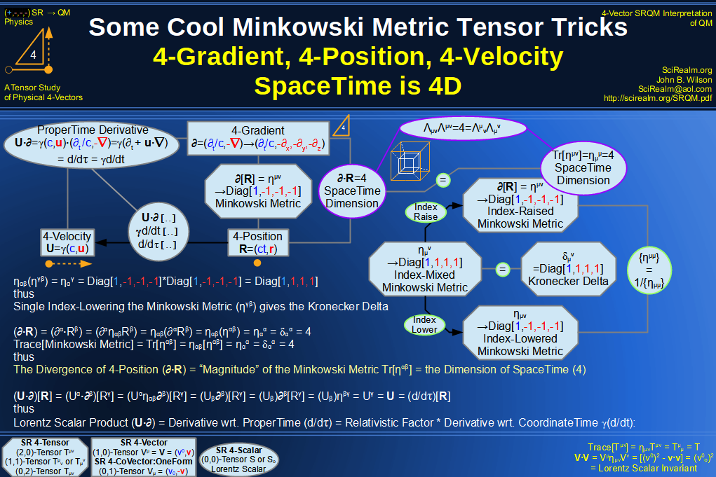
d/dτ = γ d/dt = U·∂ : Differential wrt Proper Time
Useful SR Formulas: V·V = Vo·Vo : Invariant interval is often easier to
calculate in rest frame coordinates
√[1+x] ~ (1+x/2) for x ~ 0 : Math relation often used to simplify
Relativistic eqns. to Newtonian eqns.
1/√[1+x] ~ (1-x/2) for x ~ 0 : Math relation sometimes used to simplify
Relativistic eqns. to Newtonian eqns.
δuv = Delta function = (1 if u = v, 0 if u ≠ v)
γ = (1 / √[1-(u·u/c2)]) = c/√[c2-v2]
= c/√[c2-u·u]
γ2 = c2/(c2-v2) = c2/(c2-u·u)
= 1/(1- β2)
c2/γ2 = (c2-v2)
v γ = c √[γ2-1]
β γ = √[γ2-1]
(1-β2)γ2 = 1
(1-β2) = 1/γ2
β2γ2 = γ2-1
β2γ2 +1 = γ2
β2γ = (γ-1/γ)
c2 dγ = γ3 v dv
d(γ v) = c2 dγ / v = γ3 dv
dγ = γ3 v dv / c2 = γ3 β dβ
dβ = dv / c
dγ/dv = γ3 v / c2
d(γ-1)/dv = - γ v / c2
γ' = dγ/dt = (γ3 v dv/dt)/c2 = (γ3u·a)/c2
= (u·ar)/c2
γ'' = dγ'/dt = d2γ/dt2 = (γ3/c2)*[(3γ2/c2)(u·a)2
+ (u'·a) + (u·a')] u2 = u2 u·u' = uu' = ua
(|u x a|)2 + (u·a)2 = u2a2
sin2 + cos2
= 1
(∇·∇)[1/r]
= Δ[1/r] = -4πδ3(r)
(∇·∇)[1/|r-r'|]
= Δ[1/|r-r'|] = -4πδ3(r-r') Green's function for Poisson's Eqn
SR Notation Used
**NOTE**
All results below use the time-positive SR Minkowski Metric ημν =
Diag[+1,-1,-1,-1].
If you wish to do GR, with other metrics gμν, then some results
below may need GR modification, such as the GR √[-g] for whichever metric
you are using...
You have been warned.
There are several different SR notations available that are,
mathematically speaking, equivalent.
However, some are easier to employ than others. I have used that one which
seems the most practical and least error-prone.
If you mix notations, you will get errors! Always check notation
conventions in SR & 4-Vector references, they are all relative ;-)
Minkowski SR Metric (time 0-component positive), for which {in Cartesian coordinates} ημν
= ημν = SR gμν = SR gμν = Diag[+1,-1] =
Diag[+1,-1,-1,-1]
Signature[ημν] = -2
Generic 4-Vector Definition: A = Au
= (a0,a) = (a0,a1,a2,a3) time (a0) in the 0th coord. (
some alternate notations use time as a4 )
Specific coordinate system representations: A = Au
= (a0,a) = (a0,a1,a2,a3) => (at,ax,ay,az) {for rectangular/Cartesian coords} A = Au
= (a0,a) = (a0,a1,a2,a3) => (at,ar,aθ,az) {for cylindrical coords} A = Au
= (a0,a) = (a0,a1,a2,a3) => (at,ar,aθ,aφ) {for spherical coords}
Note that the superscripted variables are not exponents, they are upper tensor indices
Intervals:
TimeLike/Temporal (+ interval) = 0 coordinate ( some alternate notations
use time as - interval and space as the + interval)
LightLike/Null (0 interval)
SpaceLike/Spatial (- interval) = 1,2,3 coordinates
Temporal Components: Future(+), Now(0), Past(-)
4-Vector Name: always references the "Spatial" 3-vector component
(basically trying to extend the Newtonian 3-vector to SR 4-vector)
4-Vector Magnitude: usually references the "temporal" scalar
component (because many vectors in the rest frame only have a temporal
component)
4-Vector Tensor Indices: I use the convention of [Greek symbols dim{0..3} = time+space], [Latin symbols dim{1..3} = only space]
4-Vector Symbols: A = Aμ = (a0,a)
= (a0,ai) = (a0,a1+a2+a3) = (a0,a1,a2,a3),
where the raised index indicates dimension, not exponent
4-Vector Definition: A = Aμ , always references the upper tensor index unless otherwise noted
4-Vector c-Factor: almost always applied to "Temporal" scalar component, as
necessary to give consistent dimensional units for all vector components
(a0,a1,a2,a3) <==>
(ct,x,y,z) = (ct,x)
*Note* c-Factor can be on the top, as ( ct , x , y , z ) = [m], or on
bottom, as ( E/c , px , py , pz ) = [kg m
s-1]. It all depends on the particular 4-Vector and its components.
*Note* P = (E/c,p) = (mc,p);
the 4-Momentum is a good case showing top or bottom, with E = mc2
4-Vector Computer HTML Representation:
SR 4-vector = {BOLD UPPERCASE} = A
time scalar component = {regular lowercase} = a0
space 3-vector component = {bold lowercase} = a = ai = (a1,a2,a3)
Contraction & Dilation Relativistic Component: v --> vo
in a rest-frame, typically v = γ vo (dilation) or v = (1/γ) vo
(contraction)
eg.
t = γ to (time dilation) - pertains to temporal separation
between two <event>'s
L = (1/γ) Lo (length contraction) - pertains to the spatial
separation between two parallel world lines
Generally, time-like quantities get dilated, space-like quantities get
contracted by motion
Also, I typically denote "at-rest" invariant quantities with a "naught",
or "o", i.e.:
Lo (invariant rest length = proper length), relativistic length
L = (1/γ) Lo
Vo (invariant rest volume), relativistic volume V = (1/γ) Vo
mo (invariant rest mass), relativistic mass m = γ mo
Eo (invariant rest energy), relativistic energy E = γ Eo
ωo (invariant rest ang-frequency), relativistic ang-frequency ω
= γ ωo
ρo (invariant rest charge-density), relativistic charge-density
ρ = γ ρo
no (invariant rest number-density), relativistic number-density
n = γ no to (invariant rest time = proper time), relativistic time
t = γ to = γ τ etc.
This avoids the confusion of some texts which use just "m" as invariant
mass, or just "ρ" as invariant charge-density.
It also helps to avoid confusion such as:
If the mass m of an object increases with velocity, wouldn't it
have be a black hole in some reference frames (near c), since the mass
increases with velocity.
Answer - no. The rest mass mo does not
change. The relativistic mass is simply an "apparent" mass, how the
object is velocity-related to an observer, not how much "stuff" is in
it...
The apparent increase is fully due to the gamma factor( γ ), which is
simply an indication of the amount of relative motion.
Imaginary unit: ( i ) used only for QM phenomena, not for SR frame
transformations or metric. To follow up on a quote from MTW " ict was put to
the sword ".
This allows all the purely SR stuff to use only real numbers.
Imaginary/complex stuff apparently only enters the scene via QM.
( some alternate notations use the imaginary unit ( i ) in the
components/frame transformations/metric )
So, in summary, this notation allows:
easy recovery of Newtonian cases by allowing (γ→1, dγ→0) when
(|v|<<c)
easy separation of SR vs Newtonian concepts, with the Newtonian 3-vector (a)
extending naturally into the SR 4-vector (A)
easy separation of SR vs QM concepts, no ict's -- ( i ) only enters into
QM concepts, such as Photon Polarization, Quantum Probability Current,
etc.
easy separation of relativistic quantities vs. invariant quantities, E = γ
Eo
reduction in number of minus signs (-), eg. U·U = c2, P·P
= (moc)2: the square magnitudes of velocity,
momentum, wavevector, and other velocity-based vectors are positive
Minkowski SR Spacetime Metric
The main assumption of SR, or GR for that matter, is that the structure
of spacetime is described by a metric gμν. A metric tells how
the spacetime is put together, or how distances are measured within the
spacetime. These distances are known as intervals. In GR, the metric may
take a number of different values, depending on various circumstances
which determine its curvature. We are interested in the
flat/pseudo-Euclidean spacetime of SR, also known as the Minkowski Metric,
for which gμν => ημν = ημν =
Diag[+1,-1,-1,-1].
"Flat" SpaceTime
ημν = gμν{SR}
t
x
y
z
t
1
0
0
0
x
0
-1
0
0
y
0
0
-1
0
z
0
0
0
-1
ημα ημβ = δαβ = (4
if α = β for Minkowski)
g = - Det[gμν] = -1 (for Minkowski) not a scalar invariant
Sqrt[-g]ρ: Scalar density
There are other ways of defining the metrics and 4-vectors available in SR
which lead to the same physical results, but this particular notation has some nice
qualities which place it above the others. First, it shows the difference
between time and space in the metric. We perceive time differently than
space, despite there being only spacetime. Also, this metric gives all of
the SR relations (frame transformations) without using the imaginary unit
( i ) in the transforms. This is important, as ( i ) is absolutely
essential for the complex wave functions once we get to QM. It is not
needed, and would only complicate and confuse matters in SR. This metric
will allow us to separate the "real" SR stuff from the "complex/imaginary"
QM stuff easily. It also allows for the possibility of complex components
in SR 4-vectors. The choice of +1 for the time component simplifies
the derived equations later on, as it allows rest-frame square-magnitudes
to be positive for most quantities of interest.
SR 4-Vector Basics
ημν = SR gμν = SR gμν =
DiagonalMatrix[1,-1,-1,-1]: Minkowski Spacetime Metric-the "flat"
spacetime of SR {in Cartesion coordinates}
A = Aμ = (a0,ai) = (a0,a1,a2,a3) => (at,ax,ay,az)
:
Typical
SR 4-vector (using all upper indices)
Aμ = (a0,ai) = (a0,a1,a2,a3) => (at,ax,ay,az) :
Typical SR 4-covector (using all lower indices)
We can always get the alternate form by applying the Minkowski Metric Tensor: Aμ
= ημνAν and Aμ = ημν Aν
Basically, this has the effect of putting a
minus sign on the space component(s)
A = Aμ = (a0,ai) = (a0,a1,a2,a3) = (a0, a1, a2, a3) = (a0,a)
:Typical
SR 4-vector (all upper indices)
Aμ = (a0,ai) = (a0,a1,a2,a3) = (a0,-a1,-a2,-a3) = (a0,-a):
Typical SR 4-covector (converted using Metric Tensor)
It is occasionally convenient to choose a particular basis to simplify component calculations
Typical bases are rectangular, cylindrical, spherical
A = Aμ = (a0,ai) = (a0,a1,a2,a3) = (a0,a) = (a0,a1,a2,a3) = (a0,a) => (at,ax,ay,az)
:Typical SR 4-vector (choosing the rectangular basis)
Aμ = (a0,ai) = (a0,a1,a2,a3) = (a0,-a) = (a0,-a1,-a2,-a3) = (a0,-a) => (at,ax,ay,az) = (at,-ax,-ay,-az)
:
Typical SR 4-covector (choosing the rectangular basis)
B = Bμ = (b0,b1,b2,b3) = (b0,b) = (bt,bx,by,bz)
:
Another
typical SR 4-vector
A·B = ημν Aμ Bν = Aν Bν
= Aμ Bμ = +a0b0-a1b1-a2b2-a3b3
= (+a0b0-a·b): The Scalar Product or Invariant Product relation,
used to make SR invariants
c(A + B) = (cA + cB) scalar multiplication A·A = A2 = (+a02 - a12
- a22 - a32) = (+a02
- a·a) magnitude squared, which can be { - , 0 , + }
A = |A| = √|A2| >= 0 absolute magnitude or
length, which can be { 0 , + } A·B = B·A commutative, with the exception of the (∂)
operator, since it only acts to the right A·(B + C) = A·B + A·C distributive
d(A·B) = d(A)·B + A·d(B)
differentiation B = d(A)/dθ, where θ is a Lorentz Scalar Invariant
Aproj = (A·B)/(B·B) B =
Projection of A along B
A|| = (A·B)/(B·B) B =
Component of A parallel to B A⊥ = A - A|| A⊥ =A - (A·B)/(B·B) B =
Component of A perpendicular to B
Let A = (a0,a) be a general 4-Vector and T = U/c = γ(c, u)/c = γ(1, β) =
(γ, γβ) be the unit-temporal 4-Vector
Then...
(A·T) = (a0,a)·γ(1, β) = γ(a0-a·β) = 1(a0o-a·0) = a0o
which is a Lorentz Invariant way to get (a0o), the rest temporal component of A
Let A = (a0,a) be a general 4-Vector and S = γβn(β·n, n) be the unit-spatial 4-Vector
Then...
-(A·S) = -(a0,a)·γβn(β·n, n) = -γβn(a0β·n, a·n) = -1(a0a·0 - a·n) = a·n
which is a Lorentz Invariant way to get (a·n), the rest spatial component of A along the n direction
If A is a time-like vector, then you can also do the following:
(A·T)2 - (A·A) = (a0o)2 - (a0a0-a·a) = (a0o)2 - (a0)2 + (a·a) = (a·a)
Sqrt[(A·T)2 - (A·A)] = Sqrt[(a·a)] = |a|
which is the Lorentz Invariant way to get the magnitude |a|, the spatial component magnitude of a time-like A
Also:
(A·A) = (a0)2 - (a·a) = invariant = (a0o)2 ,where (a0o) is the Lorentz Scalar Invariant "temporal rest value" for those vectors that can be at rest, and just the invariant for others
(a0)2 = (a0o)2 + (a·a)
Consider the f
ollowing identity:
γ = 1/Sqrt[1-β2] : γ2 = 1 + γ2β2
Multiply by the square of a Lorentz Scalar Invariant (a0o):
γ2(a0o)2 = (a0o)2 + γ2(a0o)2β2
Notice the following correspondences:
a0 = γa0o, The temporal component is the Gamma Factor times the rest value a = γa0oβ = a0β, The spatial component is temporal component times t
he Beta Factor
Try it with the 4-Momentum P = (E/c,p)
(E/c) = γ(Eo/c) or E = γEo p = γ(Eo/c)β = γ(Eo/c)(v/c) = γ(Eov/c2) = γ(mov) = γmov p = (E/c)β = (mc)β = (mv) = γmov
If β=1 then |p| = E/c or E = |p|c, which is correct for photons
It also shows that as β → 1: γ → Infinity, (a0o) → 0, a0 = (γa0o) → some finite value
Special Relativity is interesting in that it is one area of physics where {Infinity*Zero = Finite Value} for certain variables.
eg. E = γEo
For photons, the rest energy Eo = 0, the gamma factor γ = Infinity, but the overall energy of photon E = finite value for a given obs
erver.
One can do this with any SR rest value variable. Always pair γ={1..Infinity} with ao={large..0} to get a finite value a = γao={something finite}
These correspondences can also be generated by letting A = LorentzScalar (a0o) * TemporalUnit 4-Vector T A = (a0o)T = (a0o)γ(1,β) = γ(a0o)(1,β) = (γa0o)(1,β) = (a0)(1,β) = (a0,a0β) = (a0,a)
If β→0 , then A --> (a0,a0β) → (a0o,0), which has (A·A) = (a0o)2 as expected
If β→1 , then A --> (a0,a0n) → a0(1,n), which has (A·A) = (a0)2 (12 - n·n) = 0 as expected
==========
if A·A = const
then
dA1dA2dA3 / A0
dA0dA2dA3 / A1
dA0dA1dA3 / A2
dA0dA1dA2 / A3
are all scalar invariants
from Jacobian derivation
============
if Aμ dXμ = invariant for any dXμ, then Aμ
is a 4-vector
ημν Λμα Λνβ = ηαβ This is basically the reason why the Scalar Product relation gives invariants
ημν (A'μ)(B'ν) = ημν (ΛμαAα)(ΛνβBβ) = ημν (ΛμαΛνβ)(Aα)(Bβ) = ηαβ (Aα)(Bβ) = ηαβ (AαBβ)
Thus, A'·B' = A·B, where the primed 4-vectors are just Lorentz Transformed versions of the unprimed ones
Λαμ Λμβ = dαβ
A'μ = Λμν Aν: Lorentz
Transform (Transformation tensor which gives relations between alternate
boosted inertial reference frames)
Λμ'ν = (∂Xμ'/∂Xν)
Λμν = (for x-boost)
γ
-(vx/c)γ
0
0
-(vx/c)γ
γ
0
0
0
0
1
0
0
0
0
1
or
γ
-βxγ
0
0
-βxγ
γ
0
0
0
0
1
0
0
0
0
1
General Lorentz Transformation
Λμν = (for n-boost)
γ
-βxγ
-βyγ
-βzγ
-βxγ
1+(γ-1)(βx/β)2
( γ-1)(βxβy)/(β)2
( γ-1)(βxβz)/(β)2
-βyγ
( γ-1)(βyβx)/(β)2
1+( γ-1)(βy/β)2
( γ-1)(βyβz)/(β)2
-βzγ
( γ-1)(βzβx)/(β)2
( γ-1)(βzβy)/(β)2
1+( γ-1)(βz/β)2
General Lorentz Boost Transform using just vectors & components-Thank
you Jackson, Master of Vectors! Chap. 11 β = v/c, β = |β|, γ = 1/√[1-β2]
a0' = γ(a0-β·a) a' = a+(β·a)β(γ-1)/β2-γ β a0
Contraction & Dilation Relativistic Component: v --> vo
in a rest-frame, typically v = γ vo (dilation) or v = (1/γ) vo
(contraction)
eg.
t = γ to (time dilation) - pertains to temporal separation
between two <event>'s
L = (1/γ) Lo (length contraction) - pertains to the spatial
separation between two parallel world lines
Since the transformations are symmetric in the temporal and spatial parts
of the 4-vector, it is somewhat confusing how the gamma factor is
inversely related for times compared to lengths. The time dilation
compares the separation in proper time between <event>'s on the worldline of
a single particle. The length contraction is comparing separations
between differing <event>'s however. The length must be measured along
lines of simultaneity, and the <event>'s of the endpoints while simultaneous
n the rest frame, are not simultaneous in the moving frame.
We are also able to use the Rapidity
φ = Ln[γ(1+ β)] = Rapidity (which remains strictly additive in SR, unlike
v)
φ = aTanh[|p|c/E] = (1/2) Ln[(E+|p|c)/(E-|p|c)]
eφ = γ(1+β) = √[(1+β)/(1-β)]
β = Tanh[φ], γ = Cosh[φ], γβ = Sinh[φ]
φAC = φAB + φBC
Rapidity of C wrt. A = Rapidity of B wrt. A + Rapidity of C wrt. B,
provided that A,B,C are co-linear
i.e. Rapidity is strictly additive only for co-linear points
Λuv = (for x-boost, y & z
unchanged)
Cosh[φ]
-Sinh[φ]
0
0
-Sinh[φ]
Cosh[φ]
0
0
0
0
1
0
0
0
0
1
Formally, this is like a rotation in 3-space, but becomes a hyperbolic
rotation through spacetime for a Lorentz boost
Rz = (for x-y rotation about z-axis, t & z
unchanged)
1
0
0
0
0
Cos[φ]
-Sin[φ]
0
0
Sin[φ]
Cos[φ]
0
0
0
0
1
Time t = γ to --> Time Dilation (e.g. decay times of
unstable particles increase in a cyclotron)
Length L = Lo/γ --> Length Contraction
Complex SR 4-Vectors
A few 4-vectors are known to have complex components. The Polarization
4-vector and ProbabilityCurrent 4-vector are a couple of these.
It will be assumed that all physical 4-vectors may potentially be complex,
although, as far as I know, these only come into play via QM...
i = √[-1] :Imaginary Unit e0: Unit vector in the temporal direction
(typically not used since the temporal unit is always considered a scalar) e1, e2, e3
:Unit Vectors in the spatial x, y, z directions (used instead of i,
j, k so that there is no confusion with the imaginary unit
i)
Note that for the following 4-vectors, the superscript is the tensor
index, not exponentiation.
A = (a0c + a1ce1+
a2ce2+ a3ce3): Complex 4-vector has complex components, 1
along time and 3 along space
Scalar[A] = a0c: Just the time component
Vector[A] = a1ce1
+ a2ce2 + a3ce3: Just the spatial components A = Scalar[A] + Vector[A]
A = ( (a0r + a0i
) + (a1r + a1i
) e1 + (a2r
+ a2i ) e2 +
(a3r + a3i ) e3
): Complex 4-vector has real + imaginary
components, 1 each along time and 3 each along space
Re[A] = ( (a0r
) + (a1r ) e1
+ (a2r ) e2
+ (a3r ) e3
): Only the real components
Im[A] = ( (a0i
) + (a1i ) e1
+ (a2i ) e2
+ (a3i ) e3
): Only the imaginary components A = Re[A] + i Im[A]
A = (a0r + i a0i,ar
+ i ai) : Standard 4-vector A* = (a0r - i a0i,ar
- i ai): Complex conjugate 4-vector, just changes the
sign of the imaginary component
A = (a0r + i a0i,ar
+ i ai) : A* = (a0r
- i a0i,ar - i ai) B = (b0r + i b0i,br
+ i bi) : B* = (b0r
- i b0i,br - i bi)
∂·B = [( ∂/c∂tr b0r
+ ∇r·br ) - ( ∂/c∂ti b0i
+ ∇i·bi )]
+ i [( ∂/c∂tr b0i
+ ∇r·bi ) + ( ∂/c∂ti b0r
+ ∇i·br )]
= [( ∂/c∂tr b0r
+ ∇r·br ) - ( ∂/c∂ti b0i
+ ∇i·bi )]
= Re[∂·B]
The 4-Divergence of a Complex 4-Vector is Real, assuming that:
The real gradient acts only on real spaces & the imaginary gradient
acts only on imaginary spaces, thus Im[∂·B] = 0
I believe this is due to the physical functions being complex analytic
functions.
Fundamental/Universal Mathematical Constants
i = √[-1] :Imaginary Unit
π = 3.14159265358979... :Circular Const
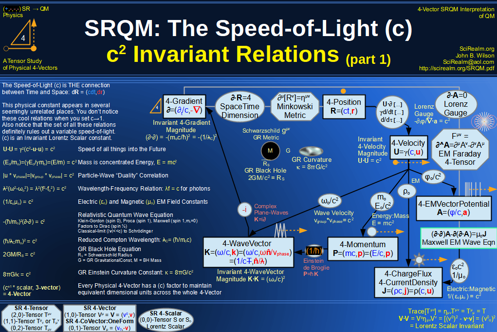
c = Speed of Light Const = 1/√[εoμo] ~ 2.99729x10⁸
[m/s]
h = Planck's Constant - relates particle to wave - Action constant
ћ = (h/2π) = Planck's Reduced Const , aka. Dirac's Const - same idea as
transforming between cycles and radians for angles
In essence, the reduced Planck constant is a conversion factor between
phase (in radians) and action (in joule-seconds)
kB = Boltzmann's Const ~ 1.3806504(24)×10−23 [J/ ºK]
relates temperature to energy
mo = Rest Mass Const (varies with particle type)
q = Electric Charge Const (varies with particle type)
Note:
I do not set various fundamental physical constants
to dimensionless unity, (i.e. c = h = G = kB = 1).
While doing so may make the mathematics/geometry a bit easier, it
ultimately obscures the physics.
While pure 4-Vectors may be Math, SR 4-Vectors is Physics. I prefer to
keep the dimensional units.
Also, it is much easier to set them to unity in a final formula than to
figure out where they go later if you need them.
Fundamental/Universal Physical SR 4-Vectors (Lorentz Vectors)
The 4-vector prototype, the "arrow" linking two <event>'s
4-Differential
dR = (cdt, dr)
dX = (cdt, dx)
[m], dt = Temporal Differential, dr
or dx = Spatial Differential, (Infinitesimals)
4-Gradient
= 4-Del or 4-Partial or 4-∇
(a vector operator)
The tensor gradient (one-form) is technically defined as
∂μ = ,μ = ∂/∂xμ = (∂t/c,∇) = (∂t/c,del)
=> (∂t/c, ∂x, ∂y, ∂z)
using the lower index
But the convention with 4-Vectors is to use upper indices
The 4-Gradient is the rare example with the upper tensor index having a negative spatial component
∂[V·R] = V, where V is not a
function of 4-position R
from QM connection:
∂ = (∂t/c, -∇)
=?= (∂t/c, β∂t/c)
=?= (vphase|-∇|/c, -∇)
The unit-temporal maybe/maybe not applies here
∂ = ∂X, as opposed to the 4-MomentumGradient ∂P
[m-1], ∂ is the partial
derivative, ∇ => (∂/∂x i + ∂/∂y j +
∂/∂z k) is the gradient operator
This is a very important 4-vector operator, often used to
generate continuity equations
Used to obtain field-kinematics
It is technically a one-form, a dual of a regular 4-vector
∂μ = ∂/∂xu = (∂/c∂t, -∇) and ∂μ = ∂/∂xu =
(∂/c∂t, ∇) ∂·∂ is also known as the D'alembertian (Wave Operator Δ)
I sometimes write out (del) because the nabla/del symbol
(∇)
is quite often displayed incorrectly in various browsers.
It should look like an inverted triangle when displayed
correctly.
Let gμ = ∂μ f = ∂f / ∂xμ
Using the chain rule, one can show:
g'ν = ∂f '/∂x'ν = Σ ( ∂f / ∂xμ
)( ∂xμ / ∂x'ν ) = ∂'ν f ' = ( ∂μ
f )( ∂'ν xμ ) = (gμ)( ∂'ν
xμ )
However, this appears to be a standard Lorentz transform
∂'μ = Λμν ∂ν[
function argument ] = ∂ν[ function argument ] Λμν
importantly: U·∂ = γ(∂/∂t + u·∇) = γ d/dt = d/dτ
The total derivative wrt. proper time is a Scalar Invariant
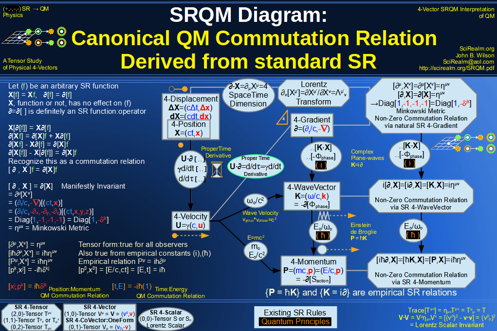
∂·X = (∂t/c,-∇)·(ct,x) = ((∂t/c)ct - (-∇·x)) = (∂tt) + (∇·x) = (1) + (3) = 4
The dimensionality of spacetime is 4.
= Diag[(∂t/c)ct, -∂xx, -∂yy, -∂zz,] = Diag[1,-1,-1,-1] = ημ
ν ∂[X] = ημν
The 4-Gradient acting on the 4-Position gives the SR Metric
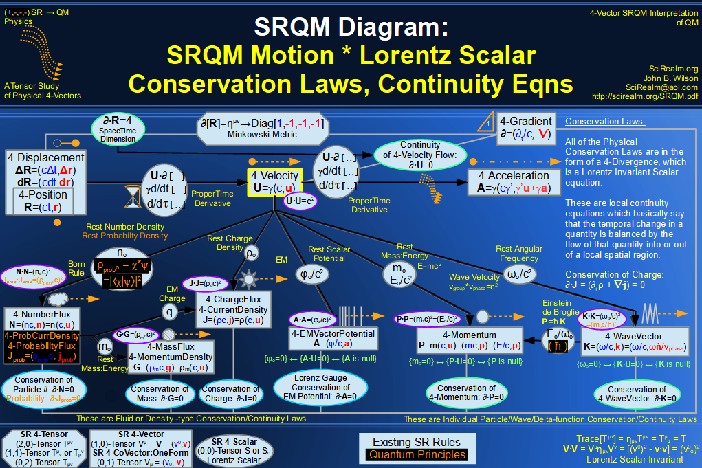
∂·J = (∂t/c,-∇)·(cρ, j) = ((∂t/c)cρ)- (-∇·j) = ∂tρ + ∇·j = 0 for a conserved ElectricCurrent
The 4-Gradient leads to various continuity eqns, which lead to various conservation eqns
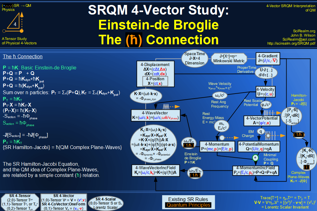
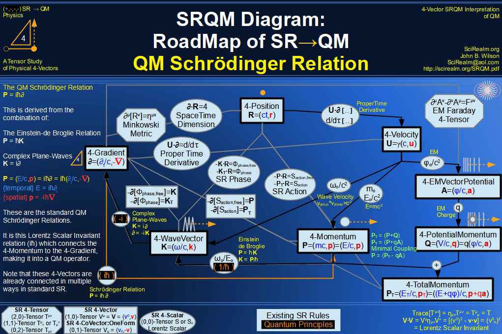
P = (E/c,p) = iћ ∂ = iћ (∂t/c, -∇)
Taking components:
Temporal: E = iћ ∂t
Spatial: p = -iћ ∇
The Schrödinger QM relations
(∂·∂)G(X|X') = δ4(X-X')
The d'Alembertian on the 4D Green's function
The 4-Gradient of a Lorentz scalar is a 4-Vector ∂[V·R] = V, where V is not a
function of R
K = (ω/c, k) R = (ct, r) K·R = -φEM = (ωt-k·r) ∂ = (∂t/c, -∇) ∂[K·R] = (∂t/c, -∇)[ωt-k·r]
= (ω/c, k) = K
*Note*
These coordinate choices do not affect the spacetime, they are
simply choices of convenience, where mathematical expressions may
take on a simpler looking form.
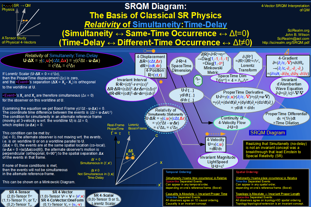
R·R = (Δs)2 = (ct)2-r·r = (ct)2-|r|2
{R·R = 0 for photonic path/null path}
{ct = |r| for photonic}
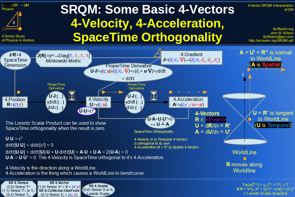
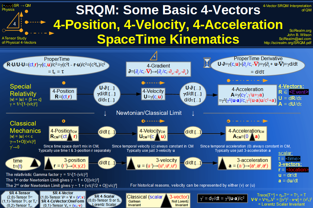
dR/dτ = U
[m], t = Time (temporal), r or x
= 3-Position (spatial)
Location of an <Event>, the most basic 4-vector (when, where)
This is just a 4-Displacement with one of the <event>'s at the
origin (0,0,0,0) of the chosen coordinate system
c = Speed-of-Light
often seen as X when choosing a Cartesian representation
often seen as R when choosing a
radial/cylindrical/spherical representation
interesting derivation: U = dR/dτ
dR = dτU R = ∫dτU
let U be a constant, then R = τU = toU
= toγ(c, u) = t(c, u) = (ct, ut)
= (ct, x)
where τ = to and t = γto
time dilation τ = t / γ
Position is essentially the ProperTime * 4-Velocity, like some
of the other flux 4-vectors
[m s-1], γ = relativistic
factor, ur = Relativistic
3-Velocity, u = dr/dt = Newtonian 3-Velocity
ur = (r)' = r' u = dr/dt = r'
thus, ur = u
"U is historically used instead of V" Uo = (c,0), 4-Velocity is always
future-pointing time-like
usually seen as U, sometimes as V
only 3 independent components since U·U = c2
= constant
the temporal component is determined by the spatial components
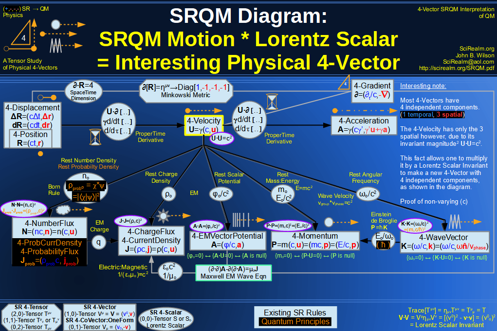
this actually gives a reason why several 4-vectors are a
(Lorentz Scalar)*(4-Velocity):
It allows these new 4-vectors to have 4 independent components
interesting derivation:
Let general 4-vector A = k U
= (ao,a) = kγ(c, u),where k is a
constant
Then A·U = k U·U
= kc2
So, ao = kγc = γ A·U / c
And, a = kγu = (γ A·U
/ c2)u = (ao/c)u
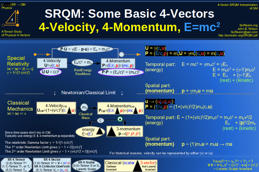
Try 4-momentum P P = (E/c,p) = moU
E/c = γ P·U /c
E = γ P·U
or, in Hamiltonian formalism, H = E = γ P·U
4-Acceleration
A = dU/dτ A = γ(c dγ/dt, dγ/dt u+γ a) = dU/dτ
= γ dU/dt
=d2R/dτ2
= γ(c dγ/dt, ar)
= γ(c γ', ar), where γ' = dγ/dt
= γ(c γ', γ' u+γ a)
= γ(ar·u/c, ar),
because
A·U = 0
= γ2[(γ2/c)(u·a), a + (γ2/c2)(u·a)
u]
Ao = (0,ao) in
rest frame
A·A = -a2
= - γ4[a2 + ( γ/c)2(u·a)2]
= - γ6[a2 - (u x a)2/c2]
[m s-2], ar
= Relativistic 3-Acceleration, a = du/dt =
Newtonian 3-Acceleration ar = (γur)' = γ'
ur + γ ur' = γ'
u + γ a = (γ3/c2)(u·a)
u + γ a a = du/dt = u'
γ' = dγ/dt = (γ3/c2)(u·a) = (u·ar)/c2
Interesting note:
The temporal component has units of frequency, before the c
factor, and is given by γ(dγ/dt)=γ(γ')
γ(c γ')=γ(u·ar)/c
γ'=(u·ar)/c2
4-Spin also has a temporal component in this form, given by u·s/c
I now wonder if all 4-vectors which are tangent to the worldline
possess this "cyclic" feature...
4-Jerk
J = dA/dτ
= γ dA/dt
=d3R/dτ3
= γ( c(dγ/dt)2 + cγ(d2γ/dt2),
dγ/dt ar+γ dar/dt
)
= γ( c γ'2 + c γ γ'', γ' ar +
γ ar' )
= γ( c γ'2 + c γ γ'', jr )
where γ' = dγ/dt, γ'' = d2γ/dt2, ar'
= dar/dt
P = ((Eo + poVo)/c2)U,
taking into account pressure*volume terms where
pressure p = po
volume V = Vo/ γ
P·P = (moc)2 = (Eo/c)2
{P·P = 0 for photonic}
dP/dτ = F
Lorentz Force - Covariant eqn. of motion for a particle in an EM
field:
dPμ / dτ = q Fμν dXν /
dτ
dPμ / dτ = q Fμν Uν
dPμ / dτ = q (∂uAν-∂νAu)Uν
4-Momentum is (moc)*UnitTemporal 4-Vector P = (moc)T
4-Momentum inc. Spin Ps = Σ·P = Σμν Pν
where Σμν is the Pauli Spin Matrix Tensor Ps = (σ0
E/c,σ·p)
where σ0
is an identity matrix of appropriate spin dimension and σ
is the Pauli Spin Matrix Vector
Ps·Ps = (σ0
E/c)2 - (σ·p)2
= (moc)2 = (Eo/c)2
4-Momentum inc. Spin in External Field
where:
H = ET = Hamiltonian = TotalEnergyOfSystem pT = Total3-MomentumOfSystem
Ps = Σ·P PT= P + qA P = PT - qA Ps = [σ0(ET/c-qφ/c)
, σ·(pT-qa)]
= (σ0
E/c,σ·p)
Note that the intrinsic spin is *not* something that must come
from QM, the spin is an artifact of the Poincare Group, where mass
and spin are the Casimir Invariants of the SR Poincare Group
[kg m s-1], E = Energy, pr
= Relativistic 3-Momentum, p = mdr/dt = Newtonian
3-Momentum
pr = p
mo = RestMass( 0 for photons, + for massive )
4-Momentum used with single whole particles
E = γmoc2 = |p|vphase
=√[(|p|c)2+(moc2)2],
in general
{E = pc, for photons}
4-Momentum is used with single whole particles
*Note* It is only the 4-Momentum of a closed system that
transforms as a 4-vector, not the 4-momenta of its open
sub-systems. For example, for a charged capacitor, one must sum
both the mechanical and EM momenta together to get an overall
4-vector for the system.
Lorentz Force - Covariant eqn. of motion for a particle in an EM
field:
dPμ / dτ = q Fμν dXν /
dτ
dPμ / dτ = q Fμν Uν
Starting with 4-Momentum inc. pressure terms... P = ((Eo + poVo)/c2)U P = (mo + poVo/c2)U P/Vo = (mo/Vo + poVo/Voc2)U P/Vo = G = (mo/Vo
+ po/c2)U G = (po_m + po/c2)U G = ((uo + po)/c2)U,
pressure p = po
g = MomentumDen = (u/c2)u = (eo)ExB,
f = g·u = MomentumFlux
u = 3-velocity, n = ParticleDen, e = EnergyPerParticle
Proper Density po_m = mo / Vo
Must be careful here though - *Note* p_m = m/V = (γmo)/(Vo/γ)
= γ2mo/Vo = γ2po_m
The mass density p_m goes as the square of γ
So this p is actually the (0,0) component of the EM
Stress Tensor
∂·G = 0 for a conserved Momentum Density, (for ex. a
perfect fluid, which is characterized by density, pressure, and
worldline velocity)
4-MomentumDensity is used with mass distributions
*Note* It is only the 4-Momentum of a closed system that
transforms as a 4-vector, not the 4-momenta of its open
sub-systems. For example, for a charged capacitor, one
must sum both the mechanical and EM momenta together to get an
overall 4-vector for the system.
U·F = γ2(dE/dt-u·fr) =
γ dmo/dt c2
(pure force if dmo/dt = 0)
solving for dE/dt, the modified rate-of-work equation
dE/dt = u·fr + c2/γ2(dmo/dτ)
dE/dt = u·fr + ( c2 - v2
)(dmo/dτ)
(Rate of particle energy change) = (rate of work done by applied
force) + (rate of work done by other mechanisms)
Let W = ( c2 - v2 )(dmo/dτ),
the work done by "non-mechanical" effects, ex. heat
In the co-moving frame,
ωo = (c2)(dmo/dτ)
Then F = γ[(fr·u + W)/c,
fr]
4-Force Density
Fd = F/Vo or
F/δVoFd = γ(du/cdt,
fdr) = dG/dτ??
[kg m-2 s-2], 4-Force
divided by rest volume element
4-ForceDensity is used with mass distributions
***Connection to Waves***
4-WaveVector
or
4-AngWaveVector
or
4-deBroglieWaveVector
K = (ωo/c)T = (ωo/c2)U
where T is the
unit-temporal 4-vector [ T
= γ(1,β) ]
[rad m-1], ω = AngularFrequency
[rad/s], k = WaveNumber or WaveVector [rad/m]
n = UnitWaveNormalVector
ω = 1/T = 2π/T AngularFreq is 2π rad/Period
k = 1/λ = 2π/λ AngularWaveNumber is 2π rad/Wavelength
T = Period T = T/2π = reduced Period
λ = Wavelength λ = λ/2π = reduced Wavelength
h = Planck's Const ћ = h/2π = reduced Planck's Const
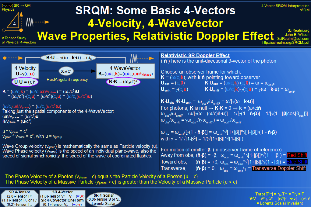
vphase = ω/k = ωλ = 1/kT = (E/ћ)/(p/ћ) = E/p = phase_velocity =
celerity = velocity of simultaneity
K = (ωo/c2)U k = (ωo/c2)γu = (γωo/c2)u
Rearranging: c2 = ωu/k = ωλu = νλu = vphase*u: True for all particles
If we let u=c, then c = ωk = ωλ = νλ = vphase: True only for photonic particles
ω2 = k2c2
+ ωo2
ω2/k2 = c2
+ ωo2/k2
vphase2 = c2 + ωo2/k2
vphase
= √[c2
+ ωo2/k2]
vgroup = dω/dk = u = <event>
velocity for SR waves
ωo = RestAngularFrequency( 0 for photons, + for
massive )
ω = 2πν, k = 2π/λ
ω = γωo k everywhere points in the direction orthogonal to planes
of constant phase φ
where phase φ = -K·R= - ( ωt - k·r ) = ( k·r
- ωt )
(d/dτ) = (U·∂) differential along 4-Velocity direction (i.e. along proper time)
(d/dθ) = (K·∂) differential along 4-Wave/Ray direction (null for photonic)
( vphase * u = c2 ) from K = (ωo/c2)U
Since (0 <= u <= c), then (c <= vphase
<=Infinity) such that ( vphase*u = c2 )
The variable u can either be taken to be the velocity of the
particle/<event> or the group velocity of the corresponding matter
wave.
ω = √[k2c2 + ωo2]
from K·K
dω/dk = (1/2)(1/√[k2 c2 + ωo2])*2kc2
= (1/ω)*kc2 = kc2/ω = c2/vphase
= u
Thus vgroup = u = vevent
vgroup = dω/dk = (∂ω/∂kx,∂ω/∂ky,∂ω/∂kz)
= u
vphase = ω/k = (ω/kx,ω/ky,ω/kz)
***this is bad notation based on our 4-vector naming
convention***
the c-factor should be in the temporal component
the 4-vector name should reference the spatial component
I simply include it here because it can sometimes be found in the literature
n = UnitWaveNormalVector
ν = ω/2π = Frequency
T = Period T = T/2π = reduced Period
λ = Wavelength λ = λ/2π = reduced Wavelength
1/λ = k/2π = Inverse WaveLength [cyc/m]
ћ = h/2π = Dirac's Const
vphase = λν = (Phase) Velocity of Wave (sometimes
called celerity)
***Flux 4-Vectors***
Flux 4-Vectors all in form of : V=
{rest_charge_density} U
V= {rest_charge}noU
where n = γno alternately, V= (cs,f)
where s = source, f= flux vector
and ∂·V = 0 for a conserved flux
Flux 4-Vectors all have units of [{charge} m-2s-1] = [{charge_density} m s-1]
Flux is the amount of {charge} that flows through a unit area
in a unit time
Flux can also be thought of as {charge_density_velocity} =
{current_density}
{charge} [{charge_unit}]
{charge_density} [{charge_units}/m3]
{flux} = {charge_density_velocity} = {current_density}
[({charge_units}/m3)*(m/s)]
= {charge per area per second}
4-NumberFlux
"SR Dust"
N = (cn, nf) = no
γ(c, u) = n(c, u)
= noU
[(#) m-2 s-1], no
= RestNumberDensity [#/m3], n = γno =
NumberDensity [#/m3] nf = nu = NumberFlux [(#/m3)*(m/s)]
# of stable particles N = noVo = nV
This is the SR "Dust" 4-Vector, which is valid for a perfect
gas,
i.e. non-interacting particles, no shear stresses, no heat
conduction
N = Σa [∫dτ δ4(x-xa(τ))(dXa/dτ)]
=
Σa [∫dτ δ4(x-xa(τ))(Ua)] ∂·N = 0 for a conserved NumberFlux
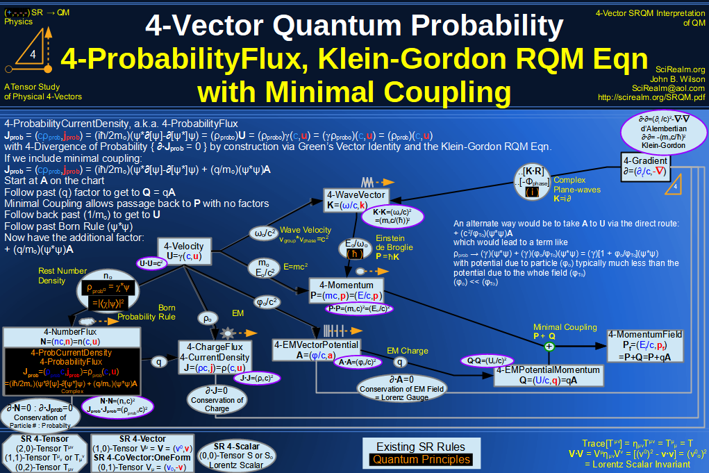
This is equivalent to 4-ProbabilityCurrentDensity
[# m-2 s-1],
4-Probability Current Density is proportional to the 4-Momentum
Equivalent to SR Dust = Number-Flux 4-vector
[(kg) m-2 s-1], u
= EnergyDen = ne, pm = MassDen = u/c2 g = MomentumDen = (u/c2)u = (eo)ExB,
f = g·u = MomentumFlux
u = 3-velocity, n = ParticleDen, e = EnergyPerParticle
Poincare' made the observation that,
since the EM momentum of radiation is 1/c2 times the
Poynting flux of energy,
radiation seems to possess a mass density 1/c2 times
its energy density
4-PoyntingVector
= 4-EnergyFlux
= 4-RadiativeFlux
= 4-MomentumDensity?
Technically not a 4-vector
Just as the (e) and (b) fields of EM are not the spatial parts of 4-vectors, the Poynting Vector (s) is not the spatial part of a 4-vector.
(s) is part of the EM Stress-Energy Tensor.
(s) is the T0i component of the symmetric EM Stress-Energy Tensor in the same way that (e) is the F0i component of the antisymmetric EM Faraday Tensor
[(J) m-2 s-1], u
= EnergyDen = ne, s = EnergyFlux = PoyntingVector = uu
= c2g = Ne ue = (εoE·E+B·B/μo)/2
=
(E·D+B·H)/2 = EM energy density
technically should be one row of the Energy-stress tensor
typically see ∂u/∂t = - ∇·s + Jf
· E
which in 4-vector notation would be ∂·S = jf
· E, where jf is the current
density of free charges, so not conserved generally
however, make the following observation:
∂[um]/∂t = j(t,x)·E(t,x),
where this is rate of change of kinetic energy of a charge
then let u = ue+um, s
= se+sm, ∂·S
= ∂[ue+um]/∂t +∇·(se+sm)
= 0
we have conservation/continuity again, by allowing energy to
transform into different types. In the example, energy is
passing back & forth between the physical charges and the EM
field itself. Energy as a whole is still conserved.
εo = Permittivity, μo = Permeability
εoμo = 1/c2 s = (E x B)/μo =
EnergyCurrentDensity u = 3-velocity, n = ParticleDen, e = EnergyPerParticle, N
= ParticleFlux = nu
see also Umov-Poynting Vector for generalization to mechanical
systems S = (cu, s) = (c(ue+um),se+sm) ∂·S = ∂[ue+um]/∂t +∇·(se+sm)
= 0 um = mechanical kinetic energy density sm = mechanical Poynting vector, the
flux of their energies
The sum of mechanical and EM energies, as well as the sum of
mechanical and EM momenta are conserved inside a closed system
of fields and charges. Another way to say this is that
only the four-momentum of a closed system transforms as a
4-vector, not the four-momentums of its open sub-systems.
Since only the microscopic fields E and B are needed in the
derivation of S = (1/μo)(ExB), assumptions about any
material possibly present can be completely avoided, and
Poynting's vector as well as the theorem in this definition are
universally valid, in vacuum as in all kinds of material. This
is especially true for the electromagnetic energy density, in
contrast to the case above
Energy types: electrical, magnetic, thermal, chemical,
mechanical, nuclear
The density of supplied energy is restricted by the physical
properties through which it flows. In a material medium, the
power of energy flux U is restricted, (U < vF), where v is
the deformation propagation velocity, usually the speed of
sound, F may be any elastic or thermal energy, U is a vector.
div U determines the amount of energy transformation into a
different form. For a gaseous medium, U = a √[T] p, where A is a
coefficient which depends on molecular composition, T is
temperature, p is pressure.
not be be confused with the 4-EntropyFlux Vector S
4-EntropyFlux
S = (cs, sf)
= so γ(c, u)
= soU
= sρoU
more correct term including heat/temp S = soU + Q/To
= sρoU + Q/To
∂·S >= 0
[(J ºK-1) m-2 s-1], so = RestEntropyDensity = qo/T, sf
= EntropyFlux
Entropy S = ∫sodV = kB ln Ω, where Ω = # of microstates for a
given macrostate
∂·S
>= 0
S
= soU
+ Q/To
where Q
is the Thermal Heat Flux 4-vector
1st term is entropy carried convectively with mass
2nd term is entropy transported by flow of heat (generalization
of dS = dQ/T)
If Q·Q
= const, then the Jacobian says that dq/qo ~ dq/T is a Scalar Invariant
β = βoU = (1/kBTo)
U
where βo = 1/kBTo
dS = β·dP,differential
entropy
* Note* This β is not the relativistic β factor
Considered on Thermodynamic
principles
also known as a Killing vector
"The proper relativistic temperature is not agreed upon by
Einstein, Ott, and Landsberg, who respectively think that moving
objects are colder, hotter and invariant. You can try reading
these and seeing what each do, how they differ in their
assumptions and why they disagree with each other. However,
given the fact that there does seem to exist genuine
disagreement, it is suspected that the matter has not been
settled. Also since neither SR nor thermodynamics are
complicated in their mathematical settings, the problem is
likely to be that of a foundational nature --- i.e. what does
temperature mean for a moving object."
4-MomentumTemperature
PT = P/kB = (pt0/c,
pT) = (T/c, pT)
= ((E/kB)/c, p/kB)
pt0 = T = Temperature (in ºK)
simply dividing 4-Momentum by Boltzmann's const. kB
which gives E/c = kBT/c, or E = kBT
Not sure if this is valid, but perhaps useful as a gauge of
photon temperature
based entirely on dimensional considerations of kB
[J/ºK] energy/temperature
similarly to c [m/s] being a fundamental constant relating
length/time
***Diffusion/Continuity based***
see
Atomic Diffusion
Brownian Motion
Electron Diffusion
Momentum Diffusion
Osmosis
Photon Diffusion
Reverse Diffusion
Thermal Diffusion
4-Potential Flux??
V = (cq, qf) = q γ(c, u)
= qU?? where q = [1]?? = ( c (k/a)φ , qf)??
= ( c (k/a)φ , -k ∇ [φ])??
needs work
Potential Flow for Velocity??
Velocity Potential
"Velocity" Conduction Equation: v = -k ∇ [φ]
"Velocity" Diffusion Equation: a ∇·∇ [φ] = ∂φ/∂t
where ∇·v ~ ∂φ/∂t
Continuity gives ∂·V = ∂[c(k/a)φ]/∂t
+∇·v = 0
Thus, [ (k/a)φ ] and [ v ] are
components of a 4-vector
In fluid dynamics, a potential flow is described by means of a
velocity potential , φ being a function of space and
time. The flow velocity v is a vector field equal
to the negative gradient, ∇, of the velocity potential φ:
Incompressible flow
In case of an incompressible flow — for instance of a liquid, or
a gas at low Mach numbers; but not for sound waves — the velocity
v has zero divergence:
∇·v = 0
with the dot denoting the inner product. As a result, the
velocity potential φ has to satisfy Laplace's equation
∇·∇φ = 0
where Δ = ∇·∇ is the Laplace operator. In this case the
flow can be determined completely from its kinematics: the
assumptions of irrotationality and zero divergence of the flow.
Dynamics only have to be applied afterwards, if one is interested
in computing pressures: for instance for flow around airfoils
through the use of Bernoulli's principle.
The flow velocity of a fluid effectively describes everything
about the motion of a fluid. Many physical properties of a fluid
can be expressed mathematically in terms of the flow velocity.
Some common examples follow:
Steady flow
Main article: Steady flow
The flow of a fluid is said to be steady if v does
not vary with time. That is if
dv/dt = 0
Incompressible flow
Main article: Incompressible flow
A fluid is incompressible if the divergence of v is zero: ∇·v = 0
That is, if v is a solenoidal
vector
field.
Irrotational flow
Main article: Irrotational
flow
A flow is irrotational if the curl
of v is zero: ∇ x v = 0 That is, if v is an irrotational
vector
field.
Vorticity
Main article: Vorticity
The vorticity, ω, of a flow can be defined in terms of
its flow velocity by
ω = ∇ x u
Thus in irrotational flow the vorticity is zero.
The velocity potential
Main article: Potential flow
If an irrotational flow occupies a simply-connected fluid region
then there exists a scalar field φ such that v = -k ∇ [φ]
The scalar field φ is called the velocity potential for the
flow. (See Irrotational vector field.)
An lamellar vector field is a synonym for an irrotational
vector field.[1] The adjective "lamellar" derives from the noun
"lamella", which means a thin layer. In Latin, lamella is
the diminutive of lamina (but do not confuse with laminar
flow). The lamellae to which "lamellar flow" refers are
the surfaces of constant potential.
An irrotational vector field which is also solenoidal is called a
Laplacian vector field.
The fundamental theorem of vector calculus states that any vector
field can be expressed as the sum of a conservative vector field
and a solenoidal field.
In vector calculus a solenoidal vector field (also known
as an incompressible vector field) is a vector field v
with divergence zero:
∇·v = 0
The fundamental theorem of vector calculus states that any vector
field can be expressed as the sum of a conservative vector field
and a solenoidal field. The condition of zero divergence is
satisfied whenever a vector field v has only a vector
potential component, because the definition of the vector
potential A as:
v = ∇ x A
automatically results in the identity (as can be shown, for
example, using Cartesian coordinates):
∇·v = ∇·(∇ x A) = 0
The converse also holds: for any solenoidal v there
exists a vector potential A such that v = ∇
x A. (Strictly speaking, this holds only subject to
certain technical conditions on v, see Helmholtz
decomposition.)
In vector calculus, a Laplacian vector field is a vector
field which is both irrotational and incompressible. If the field
is denoted as v, then it is described by the following
differential equations:
∇ x v = 0
∇·v = 0
Since the curl of v is zero, it follows that v
can be expressed as the gradient of a scalar potential (see
irrotational field) φ :
v = ∇φ (1)
Then, since the divergence of v is also zero, it follows
from equation (1) that
∇·∇φ = 0
which is equivalent to
∇2φ = 0
Therefore, the potential of a Laplacian field satisfies Laplace's
equation.
In fluid dynamics, a potential flow is a velocity field
which is described as the gradient of a scalar function: the
velocity potential. As a result, a potential flow is characterized
by an irrotational velocity field, which is a valid approximation
for several applications. The irrotationality of a potential flow
is due to the curl of a gradient always being equal to zero (since
the curl of a gradient is equivalent to take the cross product of
two parallel vectors, which is zero).
In case of an incompressible flow the velocity potential
satisfies the Laplace's equation. However, potential flows have
also been used to describe compressible flows. The potential flow
approach occurs in the modeling of both stationary as well as
nonstationary flows.
Applications of potential flow are for instance: the outer flow
field for aerofoils, water waves, and groundwater flow.
For flows (or parts thereof) with strong vorticity effects, the
potential flow approximation is not applicable.
A velocity potential is used in fluid dynamics, when a
fluid occupies a simply-connected region and is irrotational. In
such a case,
∇ x u = 0
where u denotes the flow velocity of the fluid. As a
result, u can be represented as the gradient of a scalar
function Φ:
u = ∇ Φ
Φ is known as a velocity potential for u.
A velocity potential is not unique. If a is a constant
then Φ + a is also a velocity potential for u.
Conversely, if Ψ is a velocity potential for u then Ψ = Φ
+ b for some constant b. In other words, velocity
potentials are unique up to a constant.
Unlike a stream function, a velocity potential can exist in
three-dimensional flow.
Continuity gives ∂·Q = ∂[βφP]/∂t +∇·q = 0
Thus, [ βφP ] and [ q ] are components of a 4-vector
Darcy's Law: q = -κ/μ ∇ [P]
The minus sign ensures that flux flows down the pressure
gradient
Darcy's Law - derivable from Navier-Stokes
see Fourier's law for heat conduction
see Ohm's law for electrical conduction
see Fick's law for diffusion
see Hydraulic Analogies
quantity: Volume V [m3]
potential: Pressure P [Pa] = [J/m3]
flux: Current φV [m3/s]
flux density: Velocity [m/s]
linear model: Poiseuille's Law φV = ...
4-ElectricChargeFlux
Q = (cq, qf) = q γ(c, u)
= qU = ( c ρ, j)
[(C) m-2 s-1],
Potential Flow for Charge
acts differently, presumably because this is a "charged" field,
where the particle interacts with the field.
μ = mobility
σ = specific conductivity = q n μ
where n = concentration of carriers
Fick's 1st Law Diffusion: j = - D ∇ ρ
where D = μ k T / e = Einstein-Smoluchowski Relation
Continuity independently gives ∂·J = ∂[ρ]/∂t +∇·j = 0
Thus, [ ρ ] and [ j ] are components of a 4-vector
Continuity independently gives ∂·A = ∂[φ]/∂t +∇·aEM
= 0 in the Lorenz Gauge
Thus, [ [φ ] and [ aEM
] are components of a 4-vector
Ohm's Law: j
= -σ ∇
[φ]
The minus sign ensures that current flows down the potential
gradient
see Hydraulic Analogies
quantity: Charge Q [C]
potential: Potential φ [V] = [J/C]
flux: Current I [A] = [C/s]
flux density: Current Density j [A/m2]
linear model: Ohm's Law j = - σ ∇ [φ]
***Angular Momentum/Spin/Polarization***
4-SpinMomentum
or
Pauli-Lubanski 4-vector
W = (w0,w) = (u·w/c,w)
because W·U = 0 W = (w0,w) = (p·Σ , P0Σ
+ p x k)
where Σ is the spin part of angular momentum j
W = moS
where S is the 4-Spin
[spin-momentum],
W·W = (u·w/c,w)·(u·w/c,w) = (u·w/c)2
- w·w) = - w·w = - m2 s(s+1)W2
= ( w02 - w·w ) = - (w·w) =
- (P02Σ2) = - m2c2
ћ2 s(s+1)
where Σ is the spin part of angular momentum j
(P02) = (m2c2)
(Σ2) = ћ2 s(s+1)
W·W = 0 for photonic
I am suspecting that the s(s+1) value can be derived from the Laplacian acting on a pure radial function. From mathworld.wolfram.com, ∇2[g(r)] = ∇·∇[g(r)] = (2/r)(dg/dr)+d2g/dr2
Thus, for a radial power law... ∇2[rs] = ∇·∇[rs] = (2/r)(s rs-1)+(s(s-1) rs-2) = s(s+1)rs-2
Consider that the spin 3-vector is of unit length
we get s(s+1)(1)rs-2 = s(s+1)
plays the role of covariant angular momentum
see Bargmann-Michel-Telegdi (BMT) dynamical eqn
4-Spin
S = (s0,s) = (u·s/c,s)
because S·U = 0, the spin is orthogonal to world velocity
So = (0,so) in
rest frame
S = (γ β·so , s + [γ2/(γ+1)](β·so)
β) in moving frame
S = (1/mo) W= (U·U/P·U) W
where mo = √[P·P/U·U] = P·U/U·U
Magnetic moment μ = -(g/2)(e/mc) s
U·S = 0 : 4-Spin orthogonal to worldline
dS/dτ = (-A·S/c2)U : Fermi-Walker
Transport
[ J s], = [spin] Spin =
IntrinsicAngMomentum, u·s/c = component such that U·S
= 0
4-Spin is orthogonal to 4-Velocity, so time component is zero in
rest frame So=(0,so)
This is an axial vector, or pseudovector
4-Spin has only 3 independent components, not 4, due to U·S
= 0 So=(0,so),
4-Spin is always space-like S·S = (u·s/c,s)·(u·s/c,s) =
((u·s/c)2 - s·s) = - so·so
= - ћ2 so(so+1)
Since U·S = 0
then d/dτ [U·S] = 0 = d/dτ[U]·S + U·d/dτ[S]
= A·S + U· d/dτ[S] U· d/dτ[S] = - A·S
if we assume d/dτ[S] = (k)*U then U·d/dτ[S] = kU·U = kc2 = -A·S
k = -A·S/c2
then
d/dτ[S] = (-A·S/c2)U,
which is Fermi-Walker Transport of the 4-Spin, and leads to
Thomas Precession.
Fermi-Walker Transport is the way of transporting a purely
spatial vector along the worldline of the particle in such a way
that it is as "rotationless" as possible, given that it must
remain orthogonal to the worldline.
This choice also implies that d/dτ [S·S] = 0, since d/dτ
[S·S] ~ [U·S] = 0,
which means that the magnitude of the 4-Spin is constant
=====
Thomas Precession example:
Have a particle in a circular orbit of const radius = r
(equivalent to γ'=0 and u·a = 0)
and carrying 4-Spin S
Also a chance to use cylindrical coords to simplify math
Orthonormal basis (et,er,eθ,ez)
d/dτ[(et; er; eθ;
ez)] ==> (0et; γωeθ;
-γωer; 0ez)
This gives: R = (ct, r er) U = γ(c, rω eθ) A = γ2(0, -rω2 er)
: The 4-Acceleration is highly simplified by the const r
assumption! S = (stet, srer + sθeθ + szez)
Now, match component terms et :d/dτ[st] = -γ3rω2sr/c er :d/dτ[sr] - sθγω = 0 eθ :d/dτ[sθ] + srγω = -γ3
r2ω3sr/c2 ez :d/dτ[sz] = 0
et :d/dτ[st] = -γ3 rω2sr/c er :d/dτ[sr] = sθγω eθ :d/dτ[sθ] = -γ3 r2ω3sr/c2-srγω
= -srγω(γ2 r2ω2/c2+1)
= - sr γω(γ2β2+1) = - sr
γω(γ2-1+1) = -srγ3ω ez :d/dτ[sz] = 0
Can combine the er and eθ
into harmonic equation
d2/dτ2[sr] + γ4ω2sr
= 0
sr ~ cos(Ωτ) where Ω = γ2ω
whereas orbital frequency is just ~ γω from U = γ(c, rω
eθ)
===== s·s |s,m> = ћ2 s(s+1) |s,m>
sz |s,m> = ћ m |s,m>
for s = {0 , 1/2 , 1 , 3/2 , 2 , 5/2 , ...}
for m = {-s, -s+1, ..., s-1, s}
SpinMultiplicity[m] = (2s+1) denotes the # of possible quantum
states of a system with given principal s
for s = 0, {m} = {0} singlet
for s = 1/2, {m} = {-1/2 , 1/2} doublet
for s = 1, {m} = {-1 , 0 , 1} triplet
...
|s| = ћ √[s(s+1)],
[ Sx ,Sy ] = i ћ εxyz Sz
Spin raising/lowering operators:
S± |s,m> = ћ √[s(s+1) - m(m ± 1)] |s,m> where S±
= Sx ± i Sy
Bargmann-Michel-Telegdi (BMT) dynamical eqn. for spin
dS/dτ = (e/mc)[ (g/2) FμβSβ + (1/c2)(g/2-1))vμSαFαβvβ
]
which leads to Thomas precession in the rest frame
4-SpinDensity
4-Rotation
Omega
4-Polarization
or
4-JonesVector
Ε = (ε0, ε) = (ε·u/c,ε)
for a massive particle
= (ε0, ε) = ((c/vphase) ε·n,ε)
for a wave
{E= (ε0, ε) = (ε·n,ε) ,for
light-like/photonic}
for photon travelling in z-direction
using the Jones Vector formalism n = z / |z|
E = (0,1,0,0) :
x-polarized linear E = (0,0,1,0) :
y-polarized linear E = √[1/2] (0,1,1,0) :
45 deg from x-polarized linear E = √[1/2] (0,1,i,0) :
right-polarized circular = spin 1
E = √[1/2] (0,1,-i,0) :
left-polarized circular = spin -1
General-polarized E = (0,Cos[θ]Exp[iαx],Sin[θ]Exp[iαy]),0) E* = (0,Cos[θ]Exp[-iαx],Sin[θ]Exp[-iαy]),0)
Angle θ describes the relation between the amplitudes of the
electric fields in the x and y directions
Angles αx and αy describe the phase
relationship between the wave polarized in x and the wave
polarized in y
[1], ε = PolarizationVector **This
4-vector has complex components in QM**
Called helicity for massless particles
Helicity is spin component along the direction of motion.
"Helicity is the only truly measurable component of spin for a
moving particle, but at low enough velocities
(non-relativistic), the spin component m along an external axis
becomes an alternative observable."
Like the 4-Spin, Ε orthogonal to U, or K,
so time component = 0 in rest frame
This is cancellation of the "scalar" polarization
This would again give only 3 independent components Ε·U = 0, Ε·K = 0,
Additionally, Ε·E* = -1 (normalized to unity along a
spatial direction)
Normalization combined with |u| = c for photons
is enough to reduce it to 2 independent components for photons. Ε·E* = -1 imposes
(ε·u/c)2 -ε·ε* = -1
(ε·u/c)2 -1 = -1
(ε·u/c)2 = 0 ε·u = 0, so that the spatial components must be
orthogonal.
For a massive particle, there is always a rest frame where u
= 0, so ε can have 3 independent components.
For a photonic particle, there is no rest frame.( ε·u/c
= ε·n = 0 ) is therefore an additional constraint,
limiting ε to 2 independent components, with
polarization ε orthogonal to direction of photon motion
n.
This is cancellation of the longitudinal polarization.
This seems to be related to the Ward-Takahaski Identity.
According to Wikipedia-Gauge Fixing, Many of the differences
between classical electrodynamics and QED can be accounted for
by the role that the longitudinal and time-like polarizations
play in interactions between charged particles at microscopic
distances.
see Field Quantization, by Walter Greiner, Joachim
Reinhardt
4-SpinPolarization
In the rest frame, where K = (m,0), choose a unit
3-vector n as the quantization axis.
In a frame in which the momentum is K = (k0,k)
the spin polarization of a massive particle N = Nμ
= ( k·n/m , n + (k·n) k / (m(m + k0))
) N·N = -1, Normalized to spatial unity K·N = 0,
Orthogonal to Wave Vector
alternately, S = Sμ = ( p·s/m , s
+ (p·s) p / (m(m + p0)) )
which makes more sense, called the covariant spin vector W = (w0,w) = (p·Σ , P0Σ
+ p x k)
where Σ is the spin part of angular momentum j
W2 = -m2Σ2 = -m2
s(s+1) Σ = 0 represents a spin-0 particle Σ = Dirac spinor represents a spin-1/2 particle, with Σ2
= 3/4 the unit matrix I W·N = -m Σ·n = - m s, the component of spin along n
as measured in the rest frame.
s is the spin component in the direction n that would be
measured by an observer in the particle's rest frame
Apparently this only works for massive particles, so the N
4-vector is undefined for massless
Instead, helicity h = Σ·k / |k|,
h = +1/2 or -1/2 for spin 1/2 particle
helicity is component of spin parallel to the 3-vector momentum k
w0 = (k·Σ) and k0 = |k| for a
massless particle
alternately
Nμ = ( Tμ - Pμ(pt/m2))(m/|p|)
where Tμ is the unit time-like 4-vector
I am suspecting that the s(s+1) value can be derived from the Laplacian acting on a pure radial function. From mathworld.wolfram.com, ∇2[g(r)] = ∇·∇[g(r)] = (2/r)(dg/dr)+d2g/dr2
Thus, for a radial power law... ∇2[rs] = ∇·∇[rs] = (2/r)(s rs-1)+(s(s-1) rs-2) = s(s+1)rs-2
Consider that the spin 3-vector is of unit length
we get s(s+1)(1)rs-2 = s(s+1)
4-PauliMatrix
σμ = (σ0 ,σ1 ,σ2 ,σ3)
= (σ0 ,σ) = (I ,σ)
Σ = Σμν =
Diag[σ0,-σ]??
where Σ·Σ = -2σ0??
The components of this 4-vector are
actually the Pauli Spin Matrices
So, this may actually be a 2-index tensor?? Σ = Σμν
= Diag[σ0,-σ]??
4-Momentum inc. Spin Ps = Σ·P = Σμν Pν
= ηαβ Σμα Pβ = Psμ
Σμν is a Pauli Spin Matrix Tensor = Diag[σ0,σ]
Σμν is a Pauli Spin Matrix Tensor = Diag[σ0,-σ]
The Pauli Matrices form an orthogonal basis for the complex
Hilbert space of all 2x2 matrices, meaning that any matrix M = a0σ0
+ a·σ, where A=(a0,
a) is a 4-vector
According to some books, not strictly a 4-vector, the Dirac Gamma
Matrices are actually matrices to represent intrinsic spin.
However, I have seen index raising/lowering Γμ = ημνΓμ
Γμ Γν = ημν + (1/2)σμν
σμν = [Γμ,Γν]
Not sure about a Lorentz Boost
***Electromagnetic Field Potentials***
4-VectorPotential
or
4-VectorPotentialEM
A = (φ/c, a)
4-VectorPotential of an arbitrary field
A = (φEM/c, aEM)
4-VectorPotentialEM of an EM field
technically A[R] = (φ[ct,r]/c, a[ct,r])
or A[X] = (φ[ct,x]/c, a[ct,x])
since this is field defined for all <event>'s in spacetime
I believe that in some (possibly all physical) circumstances the
following is true:
A = (φo/c2) U
A = (φ/c, a)
= (φo/c2) γ(c, u)
= (γφo/c, γφo/c2u)
giving
φ = γφo a = (γφo/c2)u
see the relativistic Lagrangian and Hamiltonian for more reasoning
for this...
For EM point charges...
AEM = (q/4πεoc) U / [R·U]ret
[..]ret implies (R·R = 0, the definition of a
light signal)
[kg m <chargetype>-1 s-1], for arbitrary field
[kg m C-1 s-1] for EM field
φEM = ScalarPotentialEM aEM = VectorPotentialEM
Electric Field E = -∇[φEM]-∂aEM/∂t
= -∇[φEM]-∂t[aEM]
Magnetic Field B = ∇ x aEM
Electric Field E [N/C = kg·m·A−1·s−3]
Magnetic Field B [Wb/m2 = kg·s−2·A−1 = N·A−1·m−1]
====
For 4-VectorPotenial of a moving point charge (Lienard-Wiechert potential) AEM = (q/4πεoc) U / [R·U]ret = (qμoc/4π)
U / [R·U]ret
where [..]ret implies (R·R = 0, the definition
of a light signal)
If we use the AEM = (φo/c2)
U definition and compare terms with
above: (φo/c2)
= (q/4πεoc) / [R·U]ret (φo) = (qc/4πεo) / [R·U]ret
(φo) = (qc/4πεo) / [c2τ]ret
(φo) = (q/4πεo)
/ [ cτ]ret
(φo) = (q/4πεo)
/ r {which is the correct potential for a point
charge in its rest frame}
since R·R = (ct)2-|r|2 = 0 --> ct = r
And likewise, the scalar and vector potential of a moving point charge
φ = (γφo) = (γq/4πεo)
/ r a = (φo/c2)γu = (γφo/c2)u = (γφo/c2)u = (φ/c2)u = ((γq/4πc2εo)
/ r)u = ((γqμo/4π)
/ r)u
If matter field is describing interaction of EM fields with
Dirac electron,
then one obtains the Maxwell eqns for QED
ρ = q ψ†ψ j = q ψ†αψ
(∂t2/c2-∇·∇)(Φ)
= μo( c2ρ ) = ( q ψ†ψ
)/εo
(∂t2/c2-∇·∇)(a)
= μo( q ψ†αψ )
If there are no sources, i.e. J = 0, then
(∂·∂)AEM
= 0
A solution to this are superpositions of polarized EM
Plane-Waves AEM = Σn [anΕ
e(i K·R)] where E is the 4-Polarization
Complex phase dθ = (q/ћ) A[X]·dX
units?(SI,guassian?)
NOTE: Neither the phase nor the components of the phase
connection are physically observable although differences in
phase connection may be observed via interference experiments.
(Ref: Aharanov-Bohm effect.)
4-Potential
***Break with standard notation***
better to use the 4-VectorPotential
Φ = (φ,c a)
Φ = (φ,c a) where Φ = cA
***this is bad notation based on our 4-vector naming
convention***
the c-factor should be in the temporal component
the 4-vector name should reference the spatial component
I simply include it here because it can sometimes be found in the literature
4-VectorPotentialGrav
4-VectorPotentialGEM
** Note **
This is an approximation only
For more accurate results the full GR theory must be used
This is just to illustrate a formal analogy between EM and Gravitational formula's in a semi-classical limit.
Agrav = (Φgrav/c, agrav)
4-VectorPotential of an arbitrary gravitational field
** Note **
This is an approximation only
For more accurate results the full GR theory must be used
This is just to illustrate a formal analogy between EM and Gravitational formula's in a semi-classical limit.
Gravitoelectromagnetism, abbreviated GEM, refers to a set of formal analogies between the equations for electromagnetism and relativistic gravitation
I believe that in some (possibly all physical) circumstances the following is true:
[kg m <chargetype>-1 s-1], for arbitrary field
[kg m <kg>-1 s-1] for GEM field
[m s-1] for GEM field
ΦGEM = ScalarPotentialGEM aGEM = VectorPotentialGEM
GravitoElectric Field Egrav = -∇[ΦGEM]-∂aGEM/∂t
= -∇[ΦGEM]-∂t[aGEM]
GravitoMagnetic Field Bgrav = ∇ x aGEM
GravitoElectric Field Egrav [m·s−2]
GravitoMagnetic Field Bgrav [s−1 ]
Jmass = (cρmass, jmass) = ρo_massU
where ρo_mass is a mass density
basically the conversion from EM to Grav is:
q --> m
εo --> -1/4πG
====
For 4-VectorPotenial of a moving point charge (Lienard-Wiechert potential) AGrav = -(Gm/c) U / [R·U]ret
where [..]ret implies (R·R = 0, the definition
of a light signal)
If we use the AGrav = (Φo_grav/c2)
U definition and compare terms with
above: (Φo_grav/c2)
= -(Gm/c) / [R·U]ret (Φo_grav) = -(Gmc) / [R·U]ret
(Φo_grav) = -(Gmc) / [c2τ]ret
(Φo_grav) = -(Gm)
/ [ cτ]ret
(Φo_grav) = -(Gm)
/ r {which is the correct potential for a point mass-charge in its rest frame}
since R·R = (ct)2-|r|2 = 0 --> ct = r
And likewise, the scalar and vector potential of a moving point mass-charge
Φgrav = (γΦo_grav) = -(γGm)
/ r a = (Φo_grav/c2)γu = (γΦo_grav/c2)u = (γΦo_grav/c2)u = (Φgrav/c2)u = -((γGm/c2)
/ r)u
[kg m s-1],
EEM = ScalarPotenialEnergy pEM = VectorPotenialMomentum
Energy and Momentum of the EM field itself, for a single charge QEM = (EEM/c, pEM)
= qoAEM
P = ћK
K = (ω/c, k) = (ω/c,ω/vphase n)
QEM = ћKEM
(for an EM field)
qo
(ΦEM/c, aEM)
= ћ(ω/c,
k)
qo ΦEM =
ћω ; qoaEM
= ћ k
4-Potential
or
4-PotentialEM ***break with standard notation***
***this is bad notation based on our 4-vector naming
convention***
the c-factor should be in the time component
the 4-vector name should reference the space component
I simply include it here because it can sometimes be found in the literature
[kg m s-1], **Momentum including
effects of potentials**
also known as Canonical Momentum
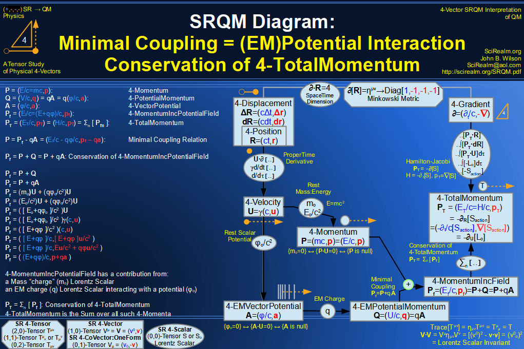
where P is the Kinetic Momentum term
where qA is the Potential Momentum term
Total Momentum = Kinetic Part + Potential Part
H = γmoc2 + q φEM pT = γmou + q aEM
Can then write dynamic momentum as P
= PT - qA
and all the usual relations still hold: P = moU = (Eo/c2)U
= ћK
4-GradientEM
Gauge Covariant Derivative
DEM = (∂/c∂t + iq/ћ ΦEM/c, -∇
+ iq/ћ aEM)
= ∂ + (iq/ћ)AEM
for electrons, commonly seen as
DEM = ∂ - (ie/ћ)AEM
where e is the electric charge
[m-1], **Gradient including
effects of EM potentials**
Minimal coupling based on principle of local gauge invariance
***Position space & Momentum Space
Differentials***
so that, in a rest frame
dVo = (1)(dVo,dVo0)
= (dVo,0)
dV = γdVo ????
V should be as follows
V = Vo/γ
Perhaps acts a little differently since this is from a
"vector-valued volume element", and not a straight volume.
Sometimes denoted as dΣμ(x)
[m3], A vector-valued volume
element is just a 4-vector that is perpendicular to all spatial
vectors in the volume element, and has a magnitude that's
proportional to the volume.
Using Clifford Algebra one can represent an oriented volume
element by a three-form. In a 4d spacetime, a 3-form has a dual
representation (Hodges Dual) which is a 1-form, which is
basically a vector.
Basically this means that you define a volume element by the
space-time vector that's perpendicular to it, and you make the
length of this space-time vector proportional to the proper
volume you wish to represent.
Hodge Duality in SR n=4 Minkowski spacetime with metric signature (+,-,-,-)
and coordinates (t,x,y,z) gives
*dt = dx^dy^dz (* is the Hodge star operator, ^ is the wedge
product operator)
alternately, dV = √[-g]d4x is an invariant volume
element scalar??
c dt dV = dx0 dx1 dx2 dx3
= dx'0 dx'1 dx'2 dx'3
c dt = dx0
dV = dx1 dx2 dx3 = d3x
(c dt)(dV) = (dx0 )(dx1 dx2 dx3)
= d4x
so that, in a rest frame
dVpo = (1)(dVpo,dVpo0) = (dVpo,0)
Sometimes denoted as dΣμ(p)
dΣμ(p) =(1/3!)ε μ ν α β dp ν x dp
α x dp β
dΣμ(p) =Pμ(d3p/p0)
[kg3 m3 s-3],
A
vector-valued MomentumSpace volume element is just a 4-vector
that is perpendicular to all spatial vectors in the
MomentumSpace volume element, and has a magnitude that's
proportional to the MomentumSpace volume.
Using the same Clifford Algebra idea from position-space, I
think this can be done
[*], Any 4-vector for which the temporal
component magnitude equals the spatial component magnitude
|a0| = |a|
which leads to the magnitude being 0, or LightLike/Photonic
ex. The 4-Velocity of a Photon, the 4-Momentum of a Photon
d[T·T]/dτ = 0 = d[T]/dτ ·T + T·d[T]/dτ
d[T]/dτ ·T = 0
Thus d[T]/dτ is orthogonal to T
[1] = dimensionless, The Unit Temporal
4-Vector
Square Magnitude = 1, Length = |1| = 1
**Interesting Formulations**
Let A=(a0,a) be a general 4-Vector
(A·T) = (a0,a)·γ(1, β) = γ(a0-a·β) = 1(a0-a·0) = a0
which is a Lorentz Invariant way to get (a0), the temporal component of A
(A·T)2 - (A·A) = (a0)2 - (a0a0-a·a) = (a0)2 - (a0)2 + (a·a) = (a·a)
Sqrt[(A·T)2 - (A·A)] = Sqrt[(a·a)] = |a|
which is the Lorentz Invariant way to get the magnitude |a|, the spatial component magnitude of A
[1] = dimensionless, A Unit Null 4-Vector
Square Magnitude = 0, Length = |0| = 0
Dependent on spatial direction n n = unit 3-vector, |n| = 1
The Null Vector is "perpendicular" to itself.
Actually not sure if "unit" null really applies here, but in
this case at least the spatial components are unit magnitude
4-Unit Spatial
4-Time Normal
S = γ[βn] (n·β,n) = (γ[βn]n·β,γ[βn]
n)
S = (s0,s)
= (s·β,s) : due to orthogonality S·T = 0
s = γ[βn] n : due to unit
magnitude S·S = -1
S = γ[βn](n·β,n) : final
form
Unit Spatial orthogonal to Unit Temporal
S·T = γ[βn](n·β,n)·γ[β](1,
β)
= γ[βn]γ[β](n·β - n·β)
= 0
A tetrad of complex, linearly-independent,
null basis vectors
Some, but not all, are orthogonal to one another
This is simply one basis, there are others
** Need to double-check these ***
see null tetrad, Sachs tetrad, Newman-Penrose tetrad
Conservation of ProbabilityCurrentDensity ∂·Jprob = ∂ρ/∂t +∇·j = 0
ρprob = γ(ψ*ψ) = γρo
See derivation of Newtonian limit below...
This is the 4-vector which relates SR to the probabilistic
formulation of QM
Derived from Klein Gordon eqn. ∂·∂ = (∂/c∂t,-∇)·(∂/c∂t,-∇)
= ∂2/c2∂t2-∇·∇ = -(moc
/ ћ)2 ∂·∂ + (moc / ћ)2 = 0
Wave eqn. on ψ, then pre-mult by ψ*
ψ*{∂·∂ + (moc / ћ)2
= 0}ψ
ψ*∂·∂ψ
+ ψ*(moc / ћ)2ψ = 0
ψ*(∂·∂ψ)
+ (moc / ћ)2ψ*ψ = 0
Wave eqn. on ψ*, then post-mult by ψ
{∂·∂ + (moc / ћ)2 = 0}ψ*ψ
(∂·∂ψ*)ψ
+ (moc / ћ)2ψ*ψ
= 0
Subtract the two
ψ*(∂·∂ψ)
+ (moc / ћ)2ψ*ψ
-(∂·∂ψ*)ψ
- (moc / ћ)2ψ*ψ
= 0
ψ*(∂·∂ψ)
- (∂·∂ψ*)ψ
= 0
Note that this is equivalent to: ∂·(ψ*∂[ψ]-∂[ψ*]ψ)
= 0
So, let Jprob ~ (ψ*∂[ψ]-∂[ψ*]ψ)
Then continuity holds ∂·Jprob = ∂ρ/∂t +∇·j
= 0
Conservation of Probability
Consider the following purely mathematical argument (based on Green's Vector Identity): ∂·( f ∂[g] - ∂[f] g ), where f and g are SR Lorentz Scalar functions
∂·( f ∂[g] - ∂[f] g )
= ∂·( f ∂[g] ) - ∂·( ∂[f] g )
= (f ∂·∂[g] + ∂[f]·∂[g]) - (∂[f]·∂[g] + ∂·∂[f] g)
= f ∂·∂[g] - ∂·∂[f] g
So, f ∂·∂[g] - ∂·∂[f] g = ∂·( f ∂[g] - ∂[f] g )
I can also multiply this by a Lorentz Invariant Scalar Constant s
s f ∂·∂[g] - ∂·∂[f] g = s ∂·( f
∂[g] - ∂[f] g ) = ∂·s( f ∂[g] - ∂[f] g )
Ok, so we have the math that we need...
Now, on to the physics... ∂·∂ = (-imoc/ћ)2 = -(moc/ћ)2: The Klein-Gordon Eqn ∂·∂ + (moc/ћ)2 = 0
Let it act on Lorentz Invariant function g ∂·∂ [g]+ (moc/ћ)2 [g] = 0 [g]
Then pre-multiply by f
[f] ∂·∂ [g]+ [f] (moc/ћ)2 [g] = [f] 0 [g]
Resulting in
[f] ∂·∂ [g]+ (moc/ћ)2[f][g] = 0
Now, do similarly with Lorentz Invariant function f ∂·∂ [f]+ (moc/ћ)2 [f] = 0 [f]
Then post-multiply by g ∂·∂ [f][g]+
(moc/ћ)2 [f][g] = 0 [f][g]
Resulting in ∂·∂ [f][g]+ (moc/ћ)2 [f][g] = 0
And as we noted from the mathematical identity at the start...
[f] ∂·∂ [g] - ∂·∂ [f][g] = ∂·( f ∂[g] - ∂[f] g ) = 0
s [f] ∂·∂ [g] - ∂·∂ [f][g] = s ∂·( f ∂[g] - ∂[f] g ) = s 0 = 0
Therefore,
s ∂·( f ∂[g] - ∂[f] g ) = 0 ∂·s( f ∂[g] - ∂[f] g ) = 0
There is a conserved current 4-vector, Jprob = s ( f ∂[g] - ∂[f] g ), for which ∂·Jprob = 0,
and which also solves the Klein-Gordon equation.
Let's choose as before (∂ = -i K) with a plane wave function f = ae^-i(K∙X), and choose g = f* = ae^i(K∙X) as it's complex conjugate.
At this point, I am going to choose s = (iћ/2mo),
which is Lorentz Scalar Invariant, in order to make the probability
have dimensionless units and be normalized to unity in the rest case.
Then Jprob = s ( f ∂[g] - ∂[f] g ) = s{f (-i) K g} - {i K f g} = s (-2i) K fg Jprob = -2is K fg Jprob = (ρprobc,jprob) = -2is K fg = -2is (ω/c,k) fg
Now, to put it in a more obvious form... f = ψ*, g = ψ
I have put off using psi until now to point out that f and g could be any kind of SR Lorentz Invariant functions.
ρprob = (γ)(&
amp;
#968;*ψ) = (γ)(ρo)
(ρo_prob) = (ψ*ψ) = fg
The probability density ρprob = γρo_prob is only equal to (ψ*ψ) in the Newtonian low-energy limiting case where γ --> 1
Thus, the Born Probability Interpretation of (ψ*ψ) only applies in the Newtonian low-energy limiting case
Jprob = s ( f ∂[g] - ∂[f] g ) = (iћ/2mo)( ψ* ∂[ψ] - ∂[ψ*] ψ ) Jprob = (iћ/2mo)( ψ* ∂[ψ] - ∂[ψ*] ψ )
Also, we know that J = ρoU and K = P/ћ = (mo/ћ)U Jprob = (ρo_prob)(ћ/mo)K Jprob = (fg)(-2is) K
So, everything matches correctly
Jcharge = qρo_probU = q(ψ*ψ)U
If we do the calculation including an EM potential, then the 4-ProbabilityCurrentDensity gains an extra component
From before: J = -2is K fg
Minimal
Coupling is just observation that the 4-TotalMomentum is the sum of the
particle 4-Momentum and the field 4-PotentialMomentum
We have conservation of the Total 4-Momentum PT PT = P + qA P = PT-qA K = KT - (q/ћ)A
Next to show Gordon Decomposition of Spin stuff...
Fundamental/Universal Relations
<Event> Tracking Relations
<Event> R
Mass mo = ρo_mVo
Energy Eo = moc2
WaveAngFreq ωo
ElecCharge q = ρoVo
MassDensity ρo_m
Mass mo = ρo_mVo
EnergyDensity uo = ρo_mc2
ChargeDensity ρo
Charge q = ρoVo
NumberDensity no
ParticleNumber No = noVo
<event>
particle
mass
wave
elec. charge
mass
density
charge
density
number
density
pos: R = (ct, r)
mo at R
ωo at R
q at R
ρo_m at R
ρo at R
no at R
vel: U = dR/dτ
P = moU = (Eo/c2)U
K = (ωo/c2)U
= (1/ћ)P
Jq =
qU
G = ρo_mU = (uo/c2)U
J = ρoU
N = noU
accel: A = dU/dτ
F= dP/dτ
Fd= dG/dτ
jerk: J = dA/dτ
snap: S = dJ/dτ
Flux 4-Vectors, 4-Vector "Charges", and the Continuity/Conservation
Equation
∂·R = (∂/c∂t,-∇)·(ct,r) = (∂/c∂t[ct]+∇·r)
= (∂/∂t[t]+∇·r) = (1+3) = 4 ∂·R = 4 The divergence of open spacetime is equal to the
number of independent dimensions (1 time + 3 space)
d/dτ [∂·R] = d/dτ [4] = 0
d/dτ [∂·R] = d/dτ [∂] · R + ∂·d/dτ [R] = d/dτ [∂] ·
R + ∂·U = γ d/dt [∂] · R + ∂·U = γ (d/dt[∂/c∂t],
-d/dt[∇])·(ct,r) + ∂·U = γ (d/dt[∂/c∂t][ct]+d/dt[∇])·r
+ ∂·U = γ (d/dt[∂/∂t][t]+d/dt[∇])·r + ∂·U =
γ (d/dt[1]+d/dt[3]) + ∂·U = 0 + ∂·U = ∂·U
thus,
∂·U = 0, which is the General SR Continuity Equation, one might say
the conservation of <event> flux or continuity of worldlines.
Due to this property, any Lorentz scalar constant times 4-Velocity U is
a conserved quantity.
For example, let N = noU, so ∂·N = ∂·noU
= no∂·U = no(0) = 0. The quantity no
is conserved.
Any "charge" constant becomes a 4-vector when multiplied by the
4-Velocity, and obeys the Conservation of Charge/Continuity equation
∂·J = ∂ρ/∂t +∇·j = 0 where J = ρoU
let Charge q = ρoVo, where ρo is the
"rest charge density", ρ = γρo is the relativistic "charge
density", Vo is the rest volume, and j = γρou
= ρu is the "ChargeDensity-Flux or Current Density"
then ChargeFlux 4-Vector = CurrentDensity 4-VectorJ = ρoU
= ρo γ(c, u) = ρ(c, u) = (cρ, j)
In the case of "electric" charge, ρo is the "rest
electric-charge density", and j is the ElectricChargedensity-flux
= electric current density
In the case of "number" charge, ρo is the "rest number-charge
density"
In the case of "mass" charge, ρo is the "rest mass density",
and j is the mass-flux = mass current density = momentum density
It can be shown that a scalar (s) and vector (v) which are related
through a continuity equation in all frames of reference (∂s/∂t + ∇·v
= 0) transform according to the Lorentz transformations and therefore
comprise the components of a 4-vector V=(cs,v), where ∂ ·V
= 0. Relativistic four-vectors may be identified from the continuity
equations of physics. See A
Proposed Relativistic, Thermodynamic Four-Vector.
Poincaré transformation or an inhomogeneous Lorentz
transformation:
ημν Λμα Λ νβ = ηαβ
Chain rule on the 4-gradient:
Let gμ = ∂μ f = ∂f / ∂xμ
Using the chain rule, one can show:
g'ν = ∂f '/∂x'ν = Σ ( ∂f / ∂xμ )( ∂xμ
/ ∂x'ν ) = ∂'ν f ' = ( ∂μ f )( ∂'ν
xμ ) = (gμ)( ∂'ν xμ )
where the brackets indicate that the gradient acts only on the function
inside the given bracket
However, this appears to be a standard Lorentz transform
∂'μ = Λμν ∂ν[function
argument] = ∂ν[function argument] Λμν
Let ∂'·J' = ∂ρ'/∂t +∇·j' = 0 be an arbitrary 4-vector
continuity equation. ∂'·J' = ημν ∂'μ J'ν = ημν
Λμα ∂α J'ν = ημν Λμα
∂α Λνβ Jβ = ημν Λμα
Λνβ ∂α Jβ = ηαβ ∂α
Jβ = ∂·J
Assuming that the 4-gradient acts only on the 4-vector J, and not on the
metric and Lorentz transforms,
which appears to be the case based on the chain rule
So, ∂'·J' = ∂·J, the continuity equations holds in arbitrary
inertial reference frames
Consider a scalar ( s ) and a vector ( v ) related by a continuity
equation, ∂s/∂t +∇·v = 0.
If this equation holds in all inertial reference frames, then s and v
must be components of a 4-vector (cs, v).
d/dτ[R] = (i ћ / mo) ∂<Event> motion ~
spacetime structure --- depends on i ћ / mo
So, the following assumptions within SR-Special Relativity lead to
QM-Quantum Mechanics:
R = (ct,r)
Location of an <event> (i.e. a particle)
within spacetime
U = dR/dτ
Velocity of the <event> is the derivative of <event> position wrt. Proper Time
P = moU
Momentum is just the Rest Mass of the
particle/<event> times its velocity
K = (1 / ћ )P
A particle's wave vector is just the
momentum divided by Dirac's constant, but uncertain by a
phase factor
∂ = -i K
The change in spacetime corresponds to (-i)
times the wave vector, whatever that means...
R·R = (Δ s)2 = (ct)2-r·r = (ct)2-|r|2
: dR·dR = (ds)2 = (c dt)2-dr·dr
= (c dt)2-|dr|2 : Invariant Interval U·U = c2 P·P = (moc)2 K·K = (moc / ћ)2 = (ωo/c)2 ∂·∂ = (∂/c∂t,-∇)·(∂/c∂t,-∇) = ∂2/c2∂t2-∇·∇
= -(moc / ћ)2 : Klein-Gordon Relativistic Wave Eqn.
Each relation may seem simple, but there is a lot of complexity generated
by each level.
*see QM from SR
(Quantum Mechanics derived from Special Relativity)*
This can be further explored: ∂·∂ + (moc / ћ)2 = 0
(∂·∂ + (moc/ћ)2
) Ψ = 0,
Ψ is a scalar Klein-Gordon eqn for massive spin-0 field
(∂·∂ + (moc/ћ)2
) A = 0
A is a 4-vector Proca eqn for massive spin-1 field
(∂·∂) Ψ = 0
Ψ is a scalar Free-wave eqn for massless (mo = 0)
spin-0 field
(∂·∂) A = 0
A is a 4-vector Maxwell eqn for massless (mo =
0) spin-1 field, no current sources
Interesting Note about Proca eqn.
"Massive charged vector field - represent with complex four-vector field φμ(X)
and impose "Lorenz condition" (∂μφμ) = 0 so that φ0(X)
-the scalar polarization- , can be discarded and the Klein-Gordon
equations emerge for the other three components φi(X)
(∂·∂ + (moc / ћ)2 ) A = 0, where A
is a 4-vector Proca eqn for massive spin-1 field
rewrite in index notation
(∂μ∂μ + (moc / ћ)2 ) Aν
= 0 and combine with the Lorenz gauge condition (∂μAμ
= 0)
apparently, this conjunction is equivalent to
∂μ( ∂μ Aν - ∂ν Aμ
)+ (moc / ћ)2 Aν = 0
which is the Euler-Lagrange equation for the Proca Action
see Conceptual Foundations of Modern Particle Physics, ~ pg. 100
Differential interval magnitude - the fundamental invariant
differential form
This is supposed to be locally valid for all <event>'s, even in GR
If we let this occur in a "rest frame", then
dRo·dRo = (c dto)2 = (c dτ)2
ΔR·ΔR = (Δs)2
= (c Δt)2-Δr·Δr = (c Δt)2-|Δr|2
Spacetime displacement interval magnitude - used to derive SR
(Δs)2 >0 TimeLike Interval(Δs)2
= 0 LightLike Interval(Δs)2 <0
SpaceLike Interval
∂·R = 4
The divergence of open spacetime is equal to the number of
independent dimensions (t,x,y,z)
K·R = -Φ = (ωt-k·r)
Phase of a SR wave; Ψ = a E e -iK·R
Photon Wave Equation (Solution to Maxwell Equation)
Part of expression used in Liénard-Wiechert potential tret = t - |x-x'|/c: (retarded
time) ru = r - r u/c = the virtual
present radius vector; i.e., the radius vector
directed from the position the charge would occupy at time t' if
it had continued with uniform velocity from its retarded position
to the field point.
ΔX·U = 0 is an interesting 4-vector condition/definition for
simultaneity
(The displacement of an external <event> is normal to either <event>'s worldline)
ΔX is a displacement vector from <Event> A to <Event> B U is an observer's 4-Velocity wrt. one of the <event>'s
The standard definition of simultaneity is when Δt = 0. This gives ΔX·U = -γ(Δx·u). But since we can always choose an observer rest frame we get ΔX·U = 0, which is thus the Lorentz Invariant condition/definition for simultaneity. However, since Δt is one of the components of a 4-vector, it is only true for certain classes of observers.
Let's examine the cases when ΔX·U = γ(c2Δt - Δx·u) = 0
then (c2Δt - Δx·u) = 0, since γ is always >=1
then (c2Δt = Δx·u)
For simultaneity, Δt = 0, therefore Δx·u = 0
if Δx = 0, then <Event> A and <Event> B are co-local, ie. at the same spatial point
if u = 0, then the observer is at rest wrt. the <Event>'s A and B
if Δx·u = 0, but Δx > 0 and u > 0, then the observer's motion must be perpendicular to a spatial line from <Event> A to <Event> B
Relations involving the 4-Velocity:
U·U = c2
The magnitude of 4-Velocity is always c2
U1·U2
= γ[u1]γ[u2](c2-u1·u2)
= γ[urel]c2
U1·U1
= U·U = c2
Relative Gamma Factor
(The scalar product of two uniformly moving <event>/particle
4-velocities is proportional to the γ factor of their relative
velocities)
Also get the relativistic addition of velocities with this:
γ[u1]γ[u2](c2-u1·u2)
= γ[urel]c2
γ1γ2(c2-u1·u2)
= γrelc2
γ1γ2(1-β1·β2)
= γrel
γ1-2γ2-2(1-β1·β2)-2
= γrel-2
(1-β1·β1)(1-β2·β2)(1-β1·β2)-2
= (1-βrel·βrel)
(βrel·βrel) = 1-(1-β1·β1)(1-β2·β2)(1-β1·β2)-2
(βrel)2 = [(1-β1·β2)2-(1-β1·β1)(1-β2·β2)](1-β1·β2)-2
(βrel)2 = [(β1)2-2(β1·β2)+(β2)2](1-β1·β2)-2
(βrel)2 = [(β1)-(β2)]2(1-β1·β2)-2 βrel = [β1-β2]/(1-β1·β2)
urel = [u1-u2]/(1-β1·β2)
or, by letting u2 --> -u2
(β2 --> -β2) urel = [u1+u2]/(1+β1·β2)
= [u1+u2]/(1+u1·u2/c2)
A1·U1 = 0,
where A is dU/dτ
The 4-Acceleration of a given particle is always normal to its
own worldline
The relative energy between <event>'s 1 and 2 is a Lorentz scalar -
any observer (<event> 3) must measure the same relative energy
between <event>'s 1 and 2
If measuring the 4-Momentum and 4-Velocity of the same <event>, then
this simplifies to the rest energy of that <event>
K1·U2 = γ[u2](ω-k1·u2)
= ωrel
K1·U1 = mo/ћU1·U1
= moc2/ћ = Eo/ћ = ωo
Relative Ang. Frequency
The relative ang. frequency between <event>'s 1 and 2 is a Lorentz
scalar - any observer (<event> 3) must measure the same relative
ang. frequency between <event>'s 1 and 2
If measuring the 4-WaveVector and 4-Velocity of the same <event>,
then this simplifies to the rest ang. frequency of that <event>
let u << c, then γ ~ 1
then U·∂ = d/dτ = γ(∂/∂t + u·∇) ~ (∂/∂t + u·∇)
= d/dt ∇t(v) = (∂/∂t + u·∇) v
is the gauge covariant derivative of a fluid where v is a
velocity vector field of a fluid
∂·U = 0 (always??)
The General Continuity Equation, one might say the conservation
of <event> flux.
I believe this is true generally but it needs checking...
If true, then it is the source of all the particle / charge /
probability continuity equations
It can be shown that a scalar (s) and vector (v) which are
related through a continuity equation in all frames of reference
(∂s/∂t + ∇·v = 0) transform according to the Lorentz
transformations and therefore comprise the components of a
4-vector V=(cs,v), where ∂ ·V = 0.
Relativistic four-vectors may be identified from the continuity
equations of physics. See A
Proposed Relativistic, Thermodynamic Four-Vector.
Relations involving the 4-Acceleration:
A·A = -a2 = -γ4[a2
+ (γ/c)2(u·a)2]
Magnitude squared of acceleration
U·A = 0, where A is dU/dτ
The 4-Acceleration of a given particle is always normal to its
own worldline U·U = c2
d/dτ(U·U) = d/dτ(c2) = 0
d/dτ(U·U) = 2*(U·dU/dτ) = 2*(U·A) = 0
A·S
Part of the proportionality factor of a 4-Spin Vector
Fermi-Walker Transported in time
Would also apply to any constant spatial 3-vector that is "attached"
to a particle
Since U·S = 0
then d/dτ [U·S] = 0 = d/dτ[U]·S + U·d/dτ[S]
= A·S + U· d/dτ[S] U· d/dτ[S] = - A·S
if we assume d/dτ[S] = (k)*U
then U·d/dτ[S] = kU·U = kc2 = -A·S
k = -A·S/c2
then d/dτ[S] = (-A·S/c2)U, which is
Fermi-Walker Transport of the 4-Spin and leads to Thomas Precession.
Fermi-Walker Transport is the way of transporting a purely spatial
vector along the worldline of the particle in such a way that it is
as "rotationless" as possible, given that it must remain orthogonal
to the worldline.
This choice also implies that d/dτ [S·S] = 0, since d/dτ [S·S]
~ [U·S] = 0,
which means that the magnitude of the 4-Spin is constant
Relativistic Billiards... P + Q = P' + Q': Momenta before and
after collision generally - Conservation of 4-Momentum P·Q = P'·Q': Momenta in an elastic (rest-mass
preserving) collision - Relative velocities conserved
Momentum representation of Dirac Equation, the 4-DiracGamma Γ with
4-Momentum P
(Γ·P)Ψ= (moc)Ψ
(ΓμPμ)Ψ= (moc)Ψ
or, in operator form iћ(Γμ∂μ)Ψ=
(moc)Ψ
(γ0p0 - γ·p
)Ψ= (moc)Ψ
One can get the equivalent result using the Pauli Spin Matrix Tensor
Σ as well
4-Momentum (inc. spin) Ps =
Σ·P
Klein-Gordon Relativistic Wave Eqn.
** ∂·∂ is also known as the D'alembertian (Wave Operator)
**
Note: Solutions to the wave equation are linear and allow
superposition!
This is a general feature of the wave equation, not something that
is only from QM
∂·J = ∂ρ/∂t +∇·j = 0
Continuity Equation - Conservation of Electric Charge
No sources or sinks
Charge is neither created nor destroyed
E·K = 0
E·E* = -1
The Polarization of a photon is orthogonal to direction of wave
motion (E·K = 0) (cancellation of "scalar" polarization)
The Polarization of a photon is always unit magnitude and
space-like (E·E* = -1)(cancellation of the longitudinal
polarization)
4-WaveVector K of photon has 4 independent components, points in null direction
4-Polariztion of photon would normally have 4 independent
components also, since it is a 4 vector
However, the ( E·K = 0 ) Polarization is orthogonal to
direction of motion, places 1 constraint, reducing to 3
independent components Ε = (ε0, ε) K = (ω/c)(1,n) , for
light-like/photonic E·K = 0 = (ε0, ε)·(ω/c)(1,n) = (ω/c)(ε0
- ε·n), so
either ω = 0 {no photon} or (ε0 = ε·n)
Thus, Ε = (ε0, ε) = (ε·n,
ε), 3 independent components ε
Photon Polarization may have complex components
In addition, ( E·E* = -1 ) plus the fact that photons
don't have a rest frame, places 1 more constraint, reducing to 2
independent components for photon E·E* = (ε·u/c)(ε·u/c)* -ε·ε*
= -1
(ε·u/c)2 -1 = -1 because (ε·ε* = 1)
(ε·u/c)2 = 0 ε·u = 0, so that the spatial components must be orthogonal.
For a massive particle, there is always a rest frame where u
= 0, so ε can have 3 independent components.
For a photonic particle, there is no rest frame.( ε·u/c =
ε·n = 0 ) is therefore an additional constraint, limiting ε
to 2 independent components, with polarization ε
orthogonal to direction of photon motion n.
There is an important distinction between an invariant
quantity and a conserved quantity.
An invariant quantity has the same value wrt. all inertial systems, but
may possibly change upon physical interaction for a system of multiple particles
(e.g. a fission/fusion reaction
"redistributes" the rest masses).
A conserved quantity maintains the same value both before and after an
interaction, although the component values may appear different in
different frames.
In 4-vector notation:
An invariant quantity is a Lorentz Scalar, the dot product of two
4-Vectors, A·B = invariant = same value for all inertial
observers.
A conserved quantity is a component of a 4-Vector that has 4-Divergence =
0, ∂·V = 0.
Relativistic Invariant Quantities (Lorentz Scalars~A·B),
although perhaps there might be some that are simply just scalars...
also known as Relativistic Covariance = Relativistic
Invariance = Lorentz Invariance
Lorentz Scalars = World Scalars = Invariant Scalars = Lorentz Invariants
Any quantity involving
counting of particles or states
Entropy, Number of
particles in a volume, Number of microstates/macrostate, etc.
Differential Length of World Line
Element, the Spacetime Interval ds
ds2 = c2dτ2
dτ = √[dR·dR/U·U]
Differential Proper Time, aka. the
Eigentime differential
d/dτ = U·∂ = γ(∂/∂t + u·∇) = γ d/dt
Derivative wrt Proper Time d/dτ
d/dt = total time derivative, ∂/∂t = partial time derivative
Δ = ∂·∂ = (∂/c∂t,-∇)·(∂/c∂t,-∇)
= ∂2/c2∂t2-∇·∇
D'Alembertian/wave operator
d4x
= dx0dx1dx2dx3
= cdtdxdydz
= cdt dV
= dX·dV
√[ |g| ]d4x is always invariant
Invariant 4-volume
Spacetime position-space differential "4-volume" element
Note: may need a correction factor if not using the Minkowski
Metric
Technically only invariant for |det Λ| = 1
also, dV = c dt dA, if eg. bundle of particles sweep this
differential volume element when directed into differential
area element over differential time
d4p = dP·dVp
Spacetime momentum-space
differential "4-volume" element
d4p δ( F[E] )
d(E/c) d3p δ( F[E] )
d(E/c) δ( F[E] ) d3p
∫ d(E/c) δ( F[E] ) d3p
but δ( F[E] ) = δ( (E/c)2-p2-P·P
) ~ δ( E - Eo )/|2E|
∫ d(E/c) δ( E - Eo )/|2E| d3p
d3p/(2E) => Lorentz Invariant
need to get exact units, etc. corrected
d3p/(2E)
= p2dpdΩ/(2E)
Spacetime
phase-space differential 3-volume element, Cartesian vs. spherical
basis
dΩ =sin(θ) dθ dφ = Solid Angle Element in direction of Ω
(2E)δ3(p-p'),
(2ω)δ3(k-k')
Spacetime phase-space
differential 3-volume element, Dirac form
need to get exact units, etc. corrected
δ4(p-p') => Lorentz
Invariant
δ( E - Eo )δ3(p-p')
δ( E - Eo )δ3(p-p') / δ( F[E]
) Divide by another Lorentz invariant
δ( E - Eo )δ3(p-p') / δ( E - Eo
)/|2E|
δ( E - Eo ) |2E| δ3(p-p') / δ(
E - Eo )
|2E| δ3(p-p')
d3p/E
E d3x
d3xd3p
Iν/ν3
d3x = c dt
dA⊥ : The photons contained in a cylinder of base area
A traveling a distance dx = c dt
Iν d ν d[ cos( θ)] dφ dA⊥ dt = Energy
carried by photons in range (ν, ν+dν)
2 ν2/c2 dν d[ cos( θ)] d φ dA⊥ dt
= 2 d3pd3x / h3
(c2 Iν
)/( 2 ν2 )= Energy per mode
n = (c2 Iν )/( 2 h ν3 ) = Number
of photons per quantum state, itself an invariant
thus Iν /ν3 is invariant
u[ε,Ω]/ε3
Specific spectral
energy density over dimensionless energy cubed
Iε[Ω]/ε3
Intensity
over dimensionless energy cubed
j[ε,Ω]/ε2
Emissivity
over dimensionless energy squared
Iν/ν3
Spectral
Intensity / ν3
Lorentz Invariant related to Relativistic Beaming or Doppler
Beaming
mo = √[P·P/U·U] =
P·U/U·U
RestMass of a Particle mo
( 0 for photons, + for massive )
ρmo = mono
= (rest mass)*(rest number density)
ProperMassDensity ρmo of
a continuum in the co-moving frame of no
Density of ProperMass in Lab Frame ρm = n mo = γ
ρmo
Density of RelativeMass pm' = n m = γ2ρmo
= γ ρ
MomentumDensity = pm'v
*Note* here ' indicates {prime}, not differentiation
q = √[J·J/N·N] = J·N/N·N
RestElectricCharge of a Particle q
3-vector
so = √[-S·S] = ћ √[s(s+1)]
Spin so S·S = - so·so
= - ћ2 so(so+1)
magnetic moment
Eo = P·U = moc2
where P = moU
RestEnergy of a Particle ( 0 for
photons, + for massive )
ωo = K·U = moc2/ћ
where K = mo/ћU
RestAngFrequency of a Particle ( 0
for photons, + for massive )
*** Phase of a wave ***,
e.g. an EM wave, a plane wave, a de Broglie matter wave...
The standard Phase (Φ) is related to the 4-WaveVector K
Φ = -K·R
The TotalPhase (ΦT) is related to the 4-TotalWaveVector KT 4-TotalMomentum PT = P + qA = ћKT = ћ(K + qA) KT = K + (q/ћ)A = (ωT/c,kT) = (ω/c + (q/ћc)φ, k + (q/ћ)a)
ΦT = -KT·R = -(K + (q/ћ)A)·R = Φ + Φpot
Φpot = -(q/ћ)A·R, where the 4-VectorPotential A is typically a function of R itself
** Note - You can see the terms for the Aharonov-Bohm effect here!!!
Do not confuse the Lorentz Scalar phase (Φ) with the scalar potential (φ), the temporal component in the 4-VectorPotential
S = -(PT·R): Action is based on the 4-TotalMomentum of the whole system ∂[S] = ∂[-(PT·R)]
= -PT PT = -∂[S]
= (ET/c,pT)
= -(∂t/c,-∇)[S] = -(∂tS/c,-∇[S]) = (-∂tS/c,∇[S])
γL = d(Saction)/dτ
which gives L = (1/γ)d(Saction)/dτ
which gives L = d(Saction)/dt
Relativistic Lagrangian L * gamma
(γ)
L = dS/dt = (1/γ)dS/dτ = (1/γ)d(-PT·R)/dτ
= (-1/γ)d(PT·R)/dτ
= (-1/γ)[(dPT/dτ·R)+(PT·dR/dτ)]
= (-1/γ)[(PT·dR/dτ)]
= (-1/γ)[(PT·U)]
= - (PT·U)/γ
{dPT/dτ =
0} since the 4-TotalMomentum should be a constant
General Formula: L = dS/dt
= p·vg - H
L = ∫ L dV = ∫ L d3x = p·vg
- H = - (H - p·vg)
ex. Lagrangian of a charged particle in EM field
L = -(PEM)·U/γ
L = -(P + QEM)·U/γ
L = -(P·U + QEM·U)/γ
L = -P·U/γ - QEM·U/γ
L = -moU·U/γ - qAEM·U/γ
L = -moc2/γ - qAEM·U/γ
L = -moc2/γ - q(ΦEM/c, aEM)·γ(c,
u)/γ
L = -moc2/γ - q(ΦEM/c,aEM)·(c, u)
L = -moc2/γ - q(ΦEM - aEM·u)
L = -moc2/γ - qΦEM + qaEM·u L = -moc2/γ - qΦoEM/γ
L = -(moc2 + qΦoEM)/γ
L + H = p·u {generally}
The Hamiltonian counts the phase-changes/unit time along t
The Lagrangian counts the phase-changes/unit time along t'
The term (pv) counts the phase-changes/unit length along x
∂L/∂q' = p
L = -moc2/γ -V: Relativistic Lagrangian
function of a Particle in a Conservative Scalar Potential
However, would need to have the Vector Potential part also to
obey full Poincare Invariance
Example would be the Lagrangian of a charged particle in the EM
field
VEM = qAEM·U/γ:
Potential of EM field
LEM = - moc2/γ - qAEM·U/γ
= - (P·P/mo + qAEM·U)/γ
= - (moU·U + qAEM·U)/γ
QED Lagrangian density
L = ψ
(i ћ c γμ Dμ - moc2)ψ
- (1/4)FμνFμν
"L = Lagrangian is the difference between kinetic and potential
energy only in the non-relativistic limit. The exact
relativistic Lagrangian is the exact total energy"
Lagrangian Eqns. of Motion, Covariant Formulation:
======================================
d/dτ[∂Lo/∂U]
= ∂Lo/∂X : Generalized
Relativistic Lagrange Eqn. (All parts are Lorentz Invariant)
Standard Lagrangian L is NOT Lorentz Invariant, just like the energy E is not Lorentz Invariant.
L = -PT·U/γ
= -(P+qA)·U/γ
Get the Rest Lagrangian Lorentz Scalar in exactly the same way we get the Rest Energy, E = γEo
Set the Lorentz Gamma Factor to 1
∂Lo/∂X
= ∂[-(P+qA)·U]/∂X = -∂[(P+qA)·U]/∂X = -∂[(P+qA)·U]/∂X = -q∂[A·U]/∂X
== -q∂[UμAμ]/∂X = -qUμ∂[Aμ]/∂X = -qUμ∂[Aμ]
assuming that the 4-Gradient of U is zero
So,
-(F+qUμ∂μ[A])
= -qUμ∂[Aμ]
(F+qUμ∂μ[A])
= qUμ∂[Aμ] F
= qUμ∂[Aμ]
- qUμ∂μ[A] F
= qUμ(∂[Aμ]
- ∂μ[A]) F
= qUμ(∂νAμ - ∂μAν)
dP/dτ = qUμ(∂νAμ
- ∂μAν)
dP/dτ = qUμFμν
L
Lagrangian Density
L = ∫ L dV = ∫ L d3x
I occasionally see the following, which is similar to the
Extended Lagrangian below
=================
Lagrangian Density for a free particle L = γL = -P·U
= - moc2
Then the Noether Charge P = -∂L/∂U = moU
which satisfies conservation law dP/dτ = 0
Let X' = X + ε: A small translation in
spacetime
then dX'/dτ = U' = dX/dτ + dε/dτ =
U + 0 = U U' = U
The Lagrangian Density is unaffected by the small spacetime
translation, so Noether's theorem applies
==================
L1 H1
Extended
Lagrangian/Hamiltonian formalism L1 = (+/-?)
-γL L1 + H1
= PT·U H1 seems to
end up being identically 0 in all frames, H1 =
H - E = 0, so I guess it is a Lorentz scalar as well
I'm not totally sure of the sign for L1, it
seems to differ in the various papers I have read on this
In any case, we have the following:
L + H = pT·u
{non-covariant, but true relativistically/Newtonian, for the
conventional Lagrangian/Hamiltonian} L1 + H1
= PT·U {covariant generally true,
for the extended Lagrangian/Hamiltonian}
L = T - V, only in Newtonian
H / γ = Pt·U
Relativistic
Hamiltonian H / gamma (γ)
Start with Lagrangian L[qi,qi'], a function
of coords qi and their time derivatives qi'
Conjugate momenta pi = ∂L/∂qi'
Then Hamiltonian H = Σ [piqi';i] - L
Then, Eqns. of Motion p' = -∂H/∂q q' = ∂H/∂p
ex. Lagrangian of a free particle
L = -moc2/γ
pi = ∂L/∂qi' = γmoui
(or p = γmou)
H = Σ [piqi';i] - L = p·u - L = γmou·u
+ moc2/γ = γmoc2
where γ2 = c2/(c2-v2)
= c2/(c2-u·u)
p' = -∂H/∂q = 0,
since H = γmoc2 has no explicit dependence
on q q' = ∂H/∂p = u
So, p' ~ a = 0
ie. no acceleration q' = u as we
expect
Hamiltonian for a free particle:
H = γmoc2 = E ; H/γ = moc2
= Eo
-------
ex. Lagrangian of a charged particle in EM field
L = -(Pt·U)/γ = { -(PEM·U)/γ
for particle in EM field }
L = -(P + QEM)·U/γ
L = -(P·U + QEM·U)/γ
L = -P·U/γ - QEM·U/γ
L = -moU·U/γ - qAEM·U/γ
L = -moc2/γ - qAEM·U/γ
L = -moc2/γ - q(ΦEM/c, aEM)·γ(c,
u)/γ
L = -moc2/γ - q(ΦEM/c,aEM)·(c, u)
L = -moc2/γ - q(ΦEM - aEM·u)
L = -moc2/γ - qΦEM + qaEM·u
L = -moc2/γ - qΦoEM/γ
L = -(moc2 + qΦoEM)/γ
this leads to the Lorentz force (here E and B are
the classical electric and magnetic fields, not 4-vectors):
pT' = f = q(E
+ v x B)
representing the rate at which the EM field adds relativistic
momentum to a charged particle
dp/dτ = γq(E + v x B)
The non-relativistic Lagrangian L is an approximation of the
relativistic one:
L = -(moc2 + qΦoEM)/γ
-L = (moc2 + qΦoEM)/γ = √[1-(v/c)2](moc2
+ qΦoEM) ~ (moc2 + qΦoEM)
- (1/2)(moc2v2/c2 + qΦoEMv2/c2)
~ (moc2 + qΦoEM) - (1/2)(mov2
+ 0)
L ~ (1/2)(mov2) - (moc2
+ qΦoEM)
L ~ (Kinetic) - (Rest+Potential) = T - V (for v << c)
The large constant coming from the restmass is simply ignored in
classical mechanics.
The gamma factor in the Lagrangian corresponds to the time
dilation of an object moving at v. In QM words: the number of
phase changes (ticks) over the trajectory of the particle
(the t' axis) is less by a factor gamma.
The non-relativistic Hamiltonian H is an approximation of the
relativistic one:
H = γ(moc2 + qΦoEM)
H = (1/√[1-(v/c)2])(moc2 + qΦoEM)
~ [1+(v/c)2/2])(moc2 + qΦoEM)
= (moc2 + qΦoEM)+(1/2)(moc2v2/c2
+ qΦoEMv2/c2) ~ (moc2
+ qΦoEM) -+(1/2)(mov2 + 0)
H ~ (1/2)(mov2) + (moc2
+ qΦoEM)
H ~ (Kinetic) + (Rest+Potential) = T + V (for v << c)
In QM words: the number of phase changes (ticks) over the t axis
is
higher by a factor gamma.
Thus, L ~ T-V and H ~ T+V only in the non-relativistic limit
(v<<c)
T = (1/2)moU·U= (1/2)P·U
??
Relativistic Kinetic Energy Term T
T = (1/2) pv
H + L = 2T = pv
non-relativistic L = T - V
but I have also seen T = (γ-1)moc2 =
γmoc2 -moc2 =
Total Energy - Rest Energy
ψ[R]
, ψ*[R]
Scalar Quantum Wave Function
A complex number which has the same value in all frames
no = √[N·N/U·U] =
N·U/U·U = n/γ
Particle RestNumberDensity (for
stat mech)
so = √[S·S/U·U] =
S·U/U·U
RestEntropyDensity (for stat mech)
Ωo = Ω
Ω = # of microstates = (N!) / (n0!n1!n2!...)
No = N
(Stable) Particle Number: N = nV =
(n/γ)(γ V) = noVo = No
n = number density, V = volume
This is an instantaneous snapshot of particle number, which is
invariant when viewed from different frames
Of course, there can be interactions which then change the
overall particle number
Po = P
Pressure of system (eg. of a tensorial perfect fluid): P = Po
So = S = kB ln Ω
Entropy: S = sV = (s/γ)(γ V) = soVo
= So ,
To = γ T
RestTemperature (according to
Einstein/Planck def.)
P =
(2q2/3c3) γ4(aperp2+
γ2a2||)
P = (μoq2a2γ6)/(6πc)
in parallel
Generally
P = μoq2(A·A)/(6πc)
Radiated
Power
P, total power is Lorentz invariant for processes with symmetry in
the rest frame
Iv/v3
Spectral
Intensity / v3
Helicity
A
massless particle moves with the speed of light,
so a real observer (who must always travel at less than the speed of light)
cannot be in any reference frame where the particle appears to
reverse its relative direction, meaning that all real observers
see the same chirality. Because of this, the direction of spin of
massless particles is not affected by a Lorentz boost
(change of viewpoint) in the direction of motion of the particle,
and the sign of the projection (helicity) is fixed for all
reference frames: the helicity is a relativistic invariant
Conserved Quantities (components of V, such
that the 4-Divergence ∂·V = 0 )
∂·J = ∂p/∂t +∇·j = 0
Conservation of 4-CurrentDensity (EM
charge): p & j change in ChargeDen wrt. time balanced by flow of CurrentDen
∂·N = ∂/∂t(γ no)+∇·(γ
nou)
= ∂n/∂t+∇·nf = 0
Conservation of 4-NumberFlux (Particle
NumberDen, NumFlux): n & nf
change in NumberDen wrt. time balanced by flow of NumFlux
∂·P = (1/c2)∂E/∂t +∇·p
= 0
Sum[Pf-Pi] = Zero
Conservation of 4-Momentum (Energy~Mass,
Momentum): E & p change in Energy wrt. time balanced by flow of Momentum
Alternately, the Sum[(Final 4-Momenta) - (Initial 4-Momenta)] =
Zero 4-Vector
Note: this conservation equation, while rarely used, is
perfectly acceptable for SR single particles. It is only when a
group of particles is treated as a continuous fluid, or motion
in GR curved space, that the Energy-Momentum (2,0)Tensor is
required. Then, the diagonal pressure terms and off-diagonal
shear terms are necessary, basically allowing statistical
particle interaction.
∂·K = ∂/c∂t(w/c)+∇·k
= (1/c2)∂w/∂t +∇·k = 0.
Conservation of 4-WaveVec (AngFreq,
WaveNum): w & k change in AngFreq wrt. time balanced by flow of WaveNum
∂·AEM = (1/c2)∂VEM/∂t
+∇·aEM = 0
Conservation of 4-VectPotentialEM
(applies in the Lorenz Gauge): VEM & aEM
change in ScalarPotential wrt. time balanced
by flow of VectorPotential
∂·U = ∂/∂t(γ[u])+∇·(γ[u] u)
= γ3 (u/c2 ∂u/∂t + ∇·u)
= ∂·Uo?
= 0 if <event> is in a conservative field or space
Conservation of 4-Velocity: (Flux-Gauss'
Law)??: γ & γ u change in (γ) wrt. time balanced by flow of (γ u)
If this quantity equals zero, then any physical quantity that is
just a (constant* 4-velocity) is conserved.
For example ∂·P = ∂·(moU) =
mo(∂·U) = 0
Also from d/dτ (∂·R) = ∂·U = 0
see also Noether's Theorem
Lorentz 4-Tensors
ημν = ημν =
Diag[1,-1,-1,-1]
= +1 if μ = ν = 0
= -1 if μ = ν = 1,2,3
= 0 if μ ≠ ν
where ρeo = rest energy density, ρmo = rest mass density,
and p = po = 0 for dust {particles do not interact}
Energy-Momentum Stress Tensor
W = Energy Density
S = Energy Flux Density?
The stress-energy tensor of a relativistic
fluid can be written in the form
Tμν = ρmoUμUν + p Hμν
+ (UμQν + QμUν) +
Πμν
Here
the world lines of the fluid elements
are the integral curves of the velocity vector Uμ,
the projection
tensor Hμν = UμUν + ημν (using ημν = Diag[-1,1,1,1]) projects other tensors onto hyperplane
elements orthogonal to Uμ,
the projection
tensor Hμν = UμUν - ημν (using ημν = Diag[1,-1,-1,-1]) projects other tensors onto hyperplane
elements orthogonal to Uμ,
the matter
density is given by the
scalar function ρmo,
the pressure is given by the Lorentz Scalar function p,
the heat
flux
vector is given by Qμ,
the viscous
shear
tensor is given by Πμν.
The heat flux vector and viscous shear
tensor are transverse to the world lines, in the sense
that
Qμ Uμ = 0, ΠμνUν = 0,
This means that they are effectively
three-dimensional quantities, and since the viscous stress
tensor is symmetric and traceless, they have respectively 3 and
5 linearly independent components. Together with the density and
pressure, this makes a total of 10 linearly independent
components, which is the number of linearly independent
components in a four-dimensional symmetric rank two tensor.
Derived Equations
*Note*
When deriving the Newtonian Limit, always use the Low Velocity
(v<<c) or Low Energy (E<<moc2)
approximations, as these apply to "real" situations
Do not use the (c --> Infinitity) approximation - while technically
making the math work, it is however an unphysical situation
4-Vector(s)
Type
Relativistic Law
Newtonian Limit
Low Velocity (v<<c) or Low Energy (E<<moc2)
Basically, β --> 0, γ --> 1
R = (ct,r)
4-Position
(ct,r) is single 4-vector entity
t and r related by Lorentz transform
t independent from r
t is independent scalar, r is independent 3-vector
ΔR = (cΔt,Δr)
4-Displacement
Relative Simultaneity
Δt' = γ(Δt - β·Δr/c)
Absolute Simultaneity
Δt' = Δt
U = dR/dτ
4-Velocity
Relativistic Composition of Velocities urel =
=[u1+u2]/(1+β1·β2)
=[u1+u2]/(1+u1·u2/c2)
Imposes Universal Speed Limit of c
Additive Velocities
u12 = u1 + u2
Unlimited Speed
A = dT/dτ
4-Acceleration
Relativistic Larmor Formula
Power radiated by moving charge
P =
= ( q2/ 6πεoc3)(A·A)
= (μoq2/6πc)(A·A)
= (μoq2/6πc) γ6/ (a2 -
(|u x a|)2/c2)
Newtonian Larmor Formula
Power radiated by a non-relativistic moving charge
P = (μoq2/6πc)(a2)
P = moU
4-Momentum
Einstein Energy-Mass Relation
E = γmoc2 = Sqrt[ mo2c4
+ p·p c2 ]
Total Energy = Rest Energy + Kinetic Energy
E = moc2 + (p2/2mo)
∂·P
Divergence of 4-Momentum
Local? Conservation of 4-Momentum
Conservation of Energy, Conservation of Momentum
P1·P2
Particle Interaction
Conservation of 4-Momentum
Conservation of Energy, Conservation of Momentum, sometimes
Conservation of Kinetic Energy
Relativistically, this is conservation of the number of worldlines
thru a given spacetime <event>
Conservation of Probability
∂·Jprob = ∂ρ/∂t +∇·j = 0
ρ = (ψ*ψ) for time separable wave functions
Typically set so that the sum over all quantum states in space = 1
At low energies/velocities, this appears as the conservation of
probability of a given wavefunction at a given spacetime <event> - In
other words, the probability interpretation of a wavefunction is
just a Newtonian approximation to the more correctly stated
conservation of relativistic worldlines. This is why the problem of
positive definite probabilities and probabilities >1 vanishes
once you consider anti-particles and conservation of charged
currents.
AEM = (ΦEM/c, aEM)
4-VectorPotential
4-VectorPotenial of a moving point charge (Lienard-Wiechert
potential)
AEM = (q/4πεoc) U / [R·U]ret
[..]ret implies (R·R = 0, the definition of a
light signal)
E2 = p·p c2 + mo2c4:
Energy of a particle has a Momentum component and a RestMass component
Total Energy: E = mc2 = γ[u] moc2 = ћω
Kinetic Energy: T = mc2-moc2 = (γ[u]-1) moc2
= (γ-1) moc2
Rest Energy: Eo = moc2
|
|___
| |
| |γ[u]
| m |
| |
|___|____
mo
Relativistic (apparent) mass m = AreaLike = γ[u] * mo = ћ w/c2
= E/c2
Theoretically, this would scale like a δ-function for photons{mo
-->0,u -->c,γ-->Infinity}
Thus, the relativistic mass of a photon is proportional to w, the angular
frequency
There is also a rest frequency ωo = moc2/ћ,
even when the massive particle is at rest. Mass is always "spinning" about
the time dimension.
U·U = c2 , d/dτ(U·U) = d/dτ(c2) = 0 ,
d/dτ(U·U) = 2*(U·dU/dτ) = 2*(U·A) = 0 U·A = 0: The 4-Acceleration is orthogonal to its own 4-Velocity
(Any acceleration is orthogonal to its own world-line, i.e. you don't
accelerate in time).
U plays the part of the tangent vector of the world-line, and A
plays the part of the normal vector of the world-line.
The curvature of a world-line is given by a/c2.
U1·U2 = γ[u1]γ[u2](c2-u1·u2)
= γ[ur]c2 (The scalar product of two uniformly
moving particles is proportional to the γ factor of their relative
velocities)
∂·R = (∂/c∂t,-∇)·(ct,r) = (∂/c∂t[ct]+∇·r)
= (∂/∂t[t]+∇·r) = (1+3) = 4 ∂·R = 4 The divergence of open space is equal to the number of
independent dimensions
d/dτ (∂·R) = d/dτ (4) = 0
d/dτ (∂·R) = d/dτ (∂) · R + ∂·d/dτ (R) = d/dτ
(∂) · R + ∂·U = γ d/dt (∂) · R + ∂·U = γ d/dt
(∂)·R + ∂·U = γ (d/dt(∂/c∂t), -d/dt(∇))·(ct,r) +
∂·U = γ (d/dt(∂/c∂t)(ct)+d/dt(∇))·r + ∂·U= γ (d/dt(∂/∂t)(t)+d/dt(∇))·r
+ ∂·U = γ (d/dt(1)+d/dt(3))+ ∂·U = ∂·U
thus,
∂·U = 0, which is the general SR continuity equation, one might say
the conservation of <event> flux. ??
Due to this property, any Lorentz scalar constant times 4-Velocity U is
a conserved quantity.
For example, let N = noU, so ∂·N =
∂·noU = no∂·U = no(0)
= 0. The quantity no is conserved.
Alternately, ∂·U = (∂/c∂t, -∇)·γ(c, u) = ∂·Uo
= (∂/c∂t, -∇)·(c, 0) = ∂/c∂t (c) = ∂/∂t (1) = 0
Relativistic Doppler Effect A = (a0, a), a generic SR 4-vector under
observation, relative to observer A·U = a Lorentz invariant, upon which all observers agree
take A·U --> A·Uo = (a0, a)·(c,0)
= ca0 = the value of the temporal component of A as
seen by observer U
now, let there be an observer Uobs at rest and
an emitter Uemit moving with respect to Uobs Uobs = (c,0): observer at rest Uemit = γ(c,v): velocity of
emitter relative to observer
--- A·Uobs = (a0, a)·(c,0)
= c a0 = ca0_obs A·Uemit = (a0, a)·γ(c,v)
= γ(ca0 - a·v)= ca0_emit
--- A·Uobs / A·Uemit = ca0_obs
/ ca0_emit = a0_obs / a0_emit A·Uobs / A·Uemit = ca0
/ γ(ca0 - a·v) = 1 / γ(1 - a·v/a0c)
= 1 / γ[1 - (|a|/a0)*(n·v/c)]
---
a0_obs / a0_emit = 1 / γ(1 - (|a|/a0)*(n·v/c))
a0_obs =
= a0_emit / γ(1 - (|a|/a0)*(n·v/c))
= a0_emit / γ(1 - (|a|/a0)*(n·β))
= a0_emit / γ(1 - (|a|/a0)*(β cos[θ]))
if A is photonic, then (|a|/a0) = 1, then a0_obs
= a0_emit / γ(1 - (n·v/c)) = a0_emit / γ(1 -
(n·β))
= a0_emit √[1+|β|]√[1-|β|] / (1 - (n·β))
thus, for photonic Doppler shifts,
if {n toward and β toward obs},
then a0_obs = a0_emit / γ[1 - |β| Cos[0°]] = a0_emit
/ γ[1 - |β|] = a0_emit √[(1+|β|)/(1-|β|)] -->Doppler
BlueShift
---
if {n toward and β 90° to obs},
then a0_obs = a0_emit / γ[1 - (|β| Cos[90°])] = a0_emit
/ γ[1 - 0] = a0_emit / γ -->the transverse Doppler
effect
---
if {n toward and β away from obs},
then a0_obs = a0_emit / γ[1 - |β| Cos[180°]] = a0_emit
/ γ[1 + |β|] = a0_emit √[(1-|β|)/(1+|β|)] -->Doppler
RedShift
Note that a0 could be any temporal component, ie. (E/c) for
4-Momentum P, (ω/c) for 4-Wavevector K, (ρc) for
4-CurrentDensity J, etc.
Commonly used notation would be the 4-frequency, for which a0 =
ν/c, leading to:
thus, for photonic frequency Doppler shifts,
if {n toward and β toward obs}, then νobs = νemit
√[(1+|β|)/(1-|β|)] -->Doppler BlueShift
if {n toward and β 90° to obs}, then νobs = νemit
/ γ -->the transverse Doppler effect
if {n toward and β away from obs}, then νobs = νemit
√[(1-|β|)/(1+|β|)] -->Doppler RedShift
Relativistic Stat-Mech (SM)/Thermodynamic stuff
U = γ(c, u), P = (E/c,p), d(P) =
(dE/c,dp) U·d(P) = γ(c dE/c-u·dp) = γ(dE-u·dp)
= γ(T dS - P dV + μ dN) = (To dSo - Po
dVo + μo dNo) = 0 ??
U·d(P) = γ(dE-u·dp) = γ(T dS - P dV +
Sum[μi dNi] + w·dL + E·dP
+ B·dM) ???
E = Energy, [Total energy of system]
u = Velocity, p = Momentum, [Translational/Kinetic energy]
T = Temperature, S = Entropy [Heat energy] P = Pressure, V = Volume [Mechanical compression energy?]
μ = Chemical Potential, N = Particle Number, ["Chemical" energy = energy
per particle] (Sum over different particle types)
w = Angular Velocity, L = Angular Momentum, [Rotational
energy] E = Electric Field, P = Polarization, [Electrical energy] B = Magnetic Field, M = Magnetization, [Magnetic energy]
Always have (intensive var * differential extensive var), intensive = sys
size independent, extensive = sys size proportional
U = γ(c, u), P = (E/c,p), U·U = c2
, P·P = (moc)2 U·P = γ(c E/c-u·p) = γ(E-u·p) = γ(T S - P V +
μ N) = (To So - Po Vo
+ μo No) ?
U·P = γ(E-u·p) = (To
So - Po Vo + μo
No) = moc2 ? for a spatially
homogeneous system: relativistic Gibbs-Duhem eqn.
Total Particle Number N = No is an invariant, because the
NumberDensity n varies as n = γ no, but this is balanced by
Volume V = Vo/γ
NumberDenstiy n = γ no where NumberFlux 4-Vector N =
(cn,nf) = no γ(c, u) = noU,no
= No/(Δ_xo*Δ_yo*Δ_zo)
N = n * V = (γ no)*(Vo/γ) = no* Vo
= No N·N = (noc)2
Total Entropy S = So is an invariant, because the
EntropyDensity s varies as s = γ so, but this is balanced by
Volume V = Vo/γ
EntropyDensity s = γ so where EntropyFlux 4-Vector S =
(cs,sf) = so γ(c, u) = soU,so
= So/(Δ_xo*Δ_yo*Δ_zo)
S = s * V = (γ so)*(Vo/γ) = so* Vo
= So S·S = (soc)2
Relativistic Analytical-Mech
Action S = S(ct,x,y,z)
dS/dτ = 0
dS/dτ = U·∂(S) = γ(∂S/∂t + u·∇(S)) = 0
see Menzel pg.172
Newtonian Approximations
√[1+x] ~ (1+x/2) for x<<1 This mathematical formula is used
to derive the Newtonian limit of the various relativistic entities
γ = (1 / √[1-(v/c)2] )
γ --> 1 for v<<c
All of the formulas below can also be generated from the 4-Velocity
Relation and multiplying by the appropriate Lorentz scalar: U·U = γ[u]2(c2-u·u) = c2
γ2(1-β·β) = 1
γ2 = 1 + γ2β2
γ = ±√[1 + γ2β2]
We choose the positive root since γ is always positive
γ = √[1 + γ2β2]
γ ~ [1 + γ2β2/2] for (γ2β2
<< 1)
4-Momentum
P = (E/c, p) P·P = (Eo/c)2 = (moc)2
E2 = Eo2 + p·p c2
E = Eo√[ 1 + p·p c2 / Eo2]
E ~ Eo( 1 + p·p c2 / 2 Eo2
+ ...) for | p·p c2 | << | Eo2
| discarding higher order terms...
E ~ ( Eo + p·p c2 / 2 Eo ) for |
p·p c2 | << | Eo2 |
E ~ ( Eo + p·p / 2 mo ) for | p·p c2
| << | Eo2 | where Eo = moc2
E ~ ( Eo + |p|2 / 2 mo ) for | p
c | << | Eo |
Total Energy = Rest Energy + Newtonian Momentum term
alternately:
γ ~ [1 + γ2β2/2]
γEo ~ Eo[1 + γ2β2/2]
E ~ [Eo + γ2Eoβ2/2]
E ~ [Eo + γ2moc2β2/2]
E ~ [Eo + γ2mo2c2β2/2mo]
E ~ [Eo + γ2mo2v2/2mo]
E ~ [Eo + p2/2mo]
4-WaveVector K = (ω/c, k) K·K = (ωo/c)2 = (Eo/ћc)2
= (moc / ћ)2
ω2 = ωo2 + k·k c2
ω = ωo √[ 1 + k·k c2 / ωo2
]
ω ~ ωo( 1 + k·k c2 / 2 ωo2
+ ...) for | k·k c2 | << | ωo2
| and choosing the positive root and discarding higher order terms...
ω ~ ( ωo + k·k c2 / 2 ωo )
for | k·k c2 | << | ωo2
|
ω ~ ( ωo + ћ k·k / 2 mo ) for | k·k
c2 | << | ωo2 | where ωo
= moc2 / ћ
ω ~ ( ωo + ћ |k|2 / 2 mo ) for | k
c | << | ωo |
Total Angular Frequency = Rest Angular Frequency + Newtonian Wave Number
term
4-Gradient (Wave equation) ∂ = ∂/∂xμ = (∂/c∂t, -∇) =
(∂t/c,
-∇) ∂·∂ = (∂to/c)2 = (- i moc / ћ )2:
Klein-Gordon Relativistic Wave eqn.
∂t2 = ∂to2 + ∇·∇
c2
∂t = ±∂to√[ 1 + ∇·∇ c2
/ ∂to2]
∂t ~ ∂to( 1 + ∇·∇ c2 /
2 ∂to2 + ...) for | ∇·∇ c2
| << | ∂to2 | and choosing the positive root
and discarding higher order terms...
∂t ~ ( ∂to + ∇·∇ c2 /
2 ∂to ) for | ∇·∇ c2 | << |
∂to2 |
∂t ~ ( ∂to - ћ ∇·∇ / i 2 mo
) for | ∇·∇ c2 | << | ∂to2
| where ∂to = - i moc2 / ћ
∂t ~ ( ∂to - ћ |∇|2 / i 2
mo ) for | ∇ c | << | ∂to |
or, in more standard form
i ћ ∂t ~ ( i ћ ∂to - ћ2 |∇|2
/ 2 mo ) for | ∇ c | << | ∂to |
where i ћ ∂to = Eo, the rest energy of the potential
V
i ћ ∂t ~ ( V(x,t) - ћ2 |∇|2
/ 2 mo ) for | ∇ c | << | ∂to |
Time dependent Schroedinger equation is just the Newtonian approximation
of the Klein-Gordon Relativistic Wave eqn.
4-ProbabilityCurrentDensity (change in form of Probability Density) J = (cρ, j) = (iћ/2mo)(ψ*∂[ψ]-∂[ψ*]ψ)
taking the temporal component, the relativistic probability density
ρ = (iћ/2moc2)(ψ* ∂t[ψ]-∂t[ψ*]
ψ)
assume wave solution in following general form:
ψ = A f [k] e(-iωt) and ψ* = A* f [k]* e(+iωt)
then
∂t[ψ] = (-iω)A f [k] e(-iωt) = (-iω)ψ and ∂t[ψ*]
= (+iω)A* f [k]* e(+iωt) = (+iω)ψ*
then
ρ = (iћ/2moc2)(ψ* ∂t[ψ]-∂t[ψ*]
ψ)
ρ = (iћ/2moc2)((-iω)ψ*ψ-(+iω)ψ*ψ)
ρ = (iћ/2moc2)((-2iω)ψ*ψ)
ρ = (ћω/moc2)(ψ*ψ)
now use the Newtonian form of ω from above
ρ ~ [ћ( ωo + ћ |k|2 / 2 mo )/moc2](ψ*ψ)
ρ ~ [(ћωo/moc2) + (ћћ
|k|2 / 2 momoc2)](ψ*ψ)
ρ ~ [(ћωo/moc2) + (ћωoћωo
|k|2c2 / 2 ωoωomoc2moc2
)](ψ*ψ)
ρ ~ [(1) + ( |k|2c2 / 2 ωo2)](ψ*ψ),
but
| k c | << | ωo |
ρ ~ [(1) + (~0)](ψ*ψ) because 2nd term is very small in
non-relativistic limit
ρ ~ (ψ*ψ)
The standard probability density (ψ*ψ) is the Newtonian
approximation of the temporal component of the 4-ProbabilityCurrent
Alternately, use ω = γωo
ρ = (ћω/moc2)(ψ*ψ)
ρ = (ћγωo/moc2)(ψ*ψ)
ρ = (γ)(ψ*ψ)
ρ ~ (ψ*ψ) where γ->1 in the Newtonian limit
The Klein-Gordon equation is more general than the Schrödinger equation,
but simplifies to the Schrödinger equation in the (φ/c)<<1 limit. ∂·∂ = (∂/c∂t,-∇)·(∂/c∂t,-∇) = ∂2/c2∂t2-∇·∇
= -(moc / ћ)2: Klein-Gordon Relativistic Wave eqn.
∂2/c2∂t2 = ∇·∇-(moc
/ ћ)2
∂2/c2∂t2 = (imoc / ћ)2+∇·∇
(i ћ)2∂2/c2∂t2 = (i ћ)2(imoc
/ ћ)2+(i ћ)2∇·∇
(i ћ)2∂2/c2∂t2 = (moc)2+(i
ћ)2∇·∇
(i ћ)2∂2/∂t2 = (moc2)2*[1
+
(i ћ/moc)2∇·∇]
(i ћ)∂/∂t = ± (moc2)*Sqrt[1 + (i ћ/moc)2∇·∇]
(i ћ)∂/∂t ~ ± (moc2)*[1 + (1/2)*(i ћ/moc)2∇·∇
+ ...] for ( ћ)2*∇·∇<<(moc)2
,generally a very good approx. for non-relativistic systems
(i ћ)∂/∂t ~ ± [(moc2) + (i2 ћ2/2mo)∇·∇
+ ...]
choosing the positive root and discarding higher order terms...
(i ћ)∂/∂t ~ (moc2) - ( ћ2/2mo)|∇|2
(i ћ)∂/∂t ~ - ( ћ2/2mo)|∇|2
becomes
the time dependent Schrödinger eqn. for a free particle
Also, extensions into EM fields (or other types of relativistic
potentials) can be made using D = ∂ + iq/ћ AEM
where AEM is the EM vector potential and q is the EM
charge,
and allowing D·D = -(moc/ћ)2 to be the more
correct EM quantum wave equation.
let A'EM = iq/ћ AEM
let M = moc/ћ then (∂ + A'EM)·(∂ + A'EM)
+ (M)2 = 0
∂·∂ + ∂·A'EM + 2 A'EM·∂ + A'EM·A'EM
+ (M)2 = 0
now the trick is that factor of 2, it comes about by keeping track of
tensor notation...
a weakness of strick 4-vector notation
let the 4-Vector potential be a conservative field, then ∂·AEM
=
0
(∂·∂) + 2(A'EM·∂) + (A'EM·A'EM)
+
(M)2 = 0
typically the vector potential a is zero in most non-relativistic settings
(i ћ)( ∂t ) ~ V[x] - (ћ)2(∇)2/2mo
And there you have it, the Schrodinger Equation with a potential
The assumptions for non-relativistic equation were:
Conservative field AEM, then ∂·AEM
=
0
(∇ + a' )2/ i2(M)2
= (∇ + a' )2/ i2(moc/ћ)2
= (ћ)2(∇ + a' )2/
i2(moc)2 is near zero
i.e. (ћ)2(∇ + a'
)2 << (moc)2, a good approximation
for low-energy systems
Arbitrarily chose vector potential a=0
Or keep it around for a near-Pauli equation (we would just have to track
spins, not included in this derivation)
Interesting Relations
(K = mo/ћU = ωo/c2 U)
gives (c2/vphasen = u) Both the
wave vector and particle velocity point in the same direction; along the
worldline. The product of the phase velocity and the particle velocity
always equals c2. ( vphase * u = c2 ). In
the case of photons, the phase velocity = particle velocity = c. In the
case of matter particles, the phase velocity vphase = c2/u
> c and particle velocity u<c. What does this mean? Suppose that you
have a collection of particles traveling at identical velocities that all
flash at the same time. The vphase is the speed at which the
flash moves in other reference frames, and can be considered the speed of
propagation of simultaneity. For particles which are at rest, the vphase
is infinite, which makes sense since they all appear to flash
simultaneously. vphase (the phase velocity) is sometimes
known as the celerity.
(∂·∂)AEM = μoJ+∂(∂·AEM)
Inhomogeneous Maxwell Equation
(∂·∂)AEM = μoJ
Homogeneous Maxwell/Lorentz Equation (if ∂·AEM
= 0 Lorenz Gauge) ∂·J = ∂ρ/∂t +∇·j = 0 Conservation of
EMcurrent Psi = a E e -iK·R Photon
Wave Equation (Solution to Maxwell Equation) E·K = 0 The Polarization of a photon is orthogonal to the
WaveVector of that photon
Fuv = ∂uAv-∂vAu
Electromagnetic Field Tensor (F0i = -Ei,Fij
= eijkBk) L = -1/4 FuvFuv -
Ju Au : Lagrangian Density for EM field
L = -moc2/γ -V: Relativistic Lagrangian function of
a Particle in a Conservative Potential
VEM = q U·AEM/γ: Potential of
EM field
LEM = -moc2/γ - q U·AEM/γ
= - (P·P/mo + qU·AEM)/γ
= - (moU·U + qU·AEM)/γ
Larmor formula can be written in Lorentz invariant form
P = -( q2/ 6πεoc3)(A·A)
=
-(μoq2)/(6πc)(A·A) Guassian units?
= ( q2/ 6πεoc3) γ6/ (u'2
- (u x u')2/c2)
= ( q2/ 6πεoc3) γ6/ (β'2
- (β x β')2)
= (2q2/ 3c(1-β'2)3) γ6/ ( β'2
- ( β x β')2) SI Units?
alternate Larmor formula:
P = (-2/3)(q2/ mo2c3)(F·F)
SI
units?
P = -( q2/ 6πεomo2c3)(F·F)
Guassian
units?
Relativistic Power radiated by moving charge by Abraham-Lorentz-Dirac
force
P = (μoq2a2γ6)/(6πc)
==== Liénard-Wiechert potentials - potential due to a moving charge
Aμ(x) = (q/c4πεo) Uμ / ( Rν Uν
) where Rν is a null vector (Rν Rν = 0)
AEM = (q/c4πεo) U / (R·U)
where (R·R = 0, the definition of a light signal)
= (q/c4πεo) U / ( cγ ( |r|-r·u/c )
)
= (q/c24π εo)(c,u)/( |r|-r·u/c )
and therefore
φEM = (q / 4 π εo ) 1/[ r - r·u/c]ret aEM = (μo q / 4 π) [u]/[ r - r·u/c]ret
where terms in square brackets [] indicate retarded quantities
(R·U) = (ct,r)·γ(c,u) = γ(c2t - r·u)
= cγ(ct - r·u/c)
tret = t - |x-x'|/c: (retarded time) ru = r - r u/c = the virtual
present radius vector; i.e., the radius vector directed
from the position the charge would occupy at time t' if it had continued
with uniform velocity from its retarded position to the field point.
=====
F = - grad V(x): Particle moving in conservative
force field
mc2 + V(x) = E = const: Relativistic energy conservation in
conservative force fields
T = mc2-moc2 = (γ[u]-1) moc2
= (γ-1) moc2 Relativistic Kinetic Energy: F·dX/dt = dT/dt: Also holds in Relativistic Mechanics F·U = (moA+(dmo/dτ)U)·U
= c2(dmo/dτ) = γc2(dmo/dt)
Relativistic Perfect Fluids, where dissipative effects (viscosity,
heat conduction, etc.) are neglected.
Particle 4-Flow N is a conservative quantity whose balance eqn. is ∂·N
= 0 N = (cn, nf) = no
γ(c, u) = n(c, u) = noU ∂·N = ∂n/∂t +∇·(nu) = 0, where n=no
γ ∂·N = ∂no γ/∂t +∇·(no γu) = 0
In non-relativistic limit this becomes ∂no/∂t
+∇·( nou) = 0
Tαβ = ((ne+p)/c2)Uα Uβ - p ηαβ
∂βTαβ = 0,
Consevation of Energy-Momentum Tensor
Everyday Special Relativistic Effects
Since the speed of light is so large, it is difficult to come up with some
ordinary type phenomena that rely on SR. There are a few, however.
Relativistic quantum chemistry:
The yellowish color of the elements gold and cesium, which would otherwise
be silvery/white : http://www.fourmilab.ch/documents/golden_glow/
The corrosion resistance of the element gold
Low melting point of element Mercury
About 10 of the 12 volts of a car's lead-acid battery due to relativistic
effects, tin-acid batteries (similar outer orbitals) too weak
Navigation:
GPS Satellite system - Would go out of synch within minutes without the
relativistic corrections, up to about 10 km difference /day
Very slight time differences of atomic clocks carried on airliners
EM:
Homopolar/Unipolar generator/motor - solution to Faraday's Paradox : http://www.physics.umd.edu/lecdem/outreach/QOTW/arch11/q218unipolar.pdf
Relativistic electron diffraction, or any other high speed electron
experiments
Faraday's Law, where a moving magnet generates an electric field, for
instance current along a wire
A plain old electromagnet, where the magnetic field is generated by moving
electrons
Various:
Fizeau's experiment of light in moving water
Cyclotron frequency of electron in magnetic field, increased effective
mass from relativistic gamma factor
Muon travel time thru atmosphere
Magnet moving past wire loop vs. wire loop moving past magnet
In atomic physics, the fine structure describes the splitting of the
spectral lines of atoms due to 1st order relativistic corrections.
Spin-orbit splitting.
Cerenkov Radiation: Matter particles moving thru a medium at greater than
the local speed of light thru the medium emit Cerenkov radiation.
Relativity gives us fermions and Fermi-Dirac statistics and the whole
structure of matter relies on the nature of fermions.
Relativity explains low energy aspects of the microscopic structure of
matter, such as atomic spectra.
It is a general property for any interacting fermion to show spin-orbit
behavior, a consequence of Lorentz Invariance.
Magnetism as the dynamic effect of moving electrical charges.
Cathode Ray Tubes, CRT's, in old style television sets and computer
monitors, had electrons moving at up to 30% c, and the magnets controlling
the beam had to be shaped with relativistic effects accounted for.
Nuclear power: One gets the massive power amounts from fission and fusion
reactions based on the relativity, which gives magnitudes more power than
regular chemical reactions.
Sunlight: It's based on nuclear fusion, which requires relativity.
Slow moving clocks:
The measurement of time dilation at everyday speeds has been accomplished
as well. Chou et al. (2010) created two clocks each holding a single 27Al+
ion in a Paul trap. In one clock, the Al+ ion was accompanied
by a 9Be+ ion as a "logic" ion, while in the other, it was
accompanied by a 25Mg+ ion. The two clocks were situated in
separate laboratories and connected with a 75 m long, phase-stabilized
optical fiber for exchange of clock signals. These optical atomic clocks
emitted frequencies in the petahertz (1 PHz = 1015 Hz) range
and had frequency uncertainties in the 10-17 range. With these
clocks, it was possible to measure a frequency shift due to time dilation
of ~10-16 at speeds below 36 km/h (< 10 m/s, the speed of a
fast runner) by comparing the rates of moving and resting aluminum ions.
It was also possible to detect gravitational time dilation from a
difference in elevation between the two clocks of 33 cm
Things to look-up
It can be shown that a scalar (s) and vector (v) which are related
through a continuity equation in all frames of reference (∂s/∂t + ∇·v
= 0) transform according to the Lorentz transformations and therefore
comprise the components of a 4-vector V=(cs,v), where ∂ ·V
= 0. Relativistic four-vectors may be identified from the continuity
equations of physics. See A
Proposed Relativistic, Thermodynamic Four-Vector.
Also, the diffusion equation can be derived from the continuity equation,
which states that a change in density in any part of a system is due to
inflow/outflow of material into/out-of that part of the system.
Essentially, no material is created/destroyed. ∂·J = ∂p/∂t +∇·j
= 0
If j is the flux of diffusing material, then the diffusion equation is
obtained by combining continuity with the assumption that the flux of
diffusing material in any part of the system is proportional to the local
density gradient. j = - D(p) ∇p. see Fick's
law of diffusion
Not every vector field has a scalar potential; those which do are called conservative,
corresponding to the notion of conservative force in physics. Among
velocity fields, any lamellar field has a scalar potential, whereas a
solenoidal field only has a scalar potential in the special case when it
is a Laplacian field.
In vector calculus a conservative vector field is a vector field
which is the gradient of a scalar potential. There are two closely related
concepts: path independence and irrotational vector
fields. Every conservative vector field has zero curl (and is thus
irrotational), and every conservative vector field has the path
independence property. In fact, these three properties are equivalent in
many 'real-world' applications.
An lamellar vector field is a synonym for an irrotational vector
field.[1] The adjective "lamellar" derives from the noun "lamella", which
means a thin layer. In Latin, lamella is the diminutive of lamina
(but do not confuse with laminar flow). The lamellae to which
"lamellar flow" refers are the surfaces of constant potential.
An irrotational vector field which is also solenoidal is called a
Laplacian vector field.
The fundamental theorem of vector calculus states that any vector field
can be expressed as the sum of a conservative vector field and a
solenoidal field.
In vector calculus a solenoidal vector field (also known as an incompressible
vector field) is a vector field v with divergence zero:
∇·v = 0
The fundamental theorem of vector calculus states that any vector field
can be expressed as the sum of a conservative vector field and a
solenoidal field. The condition of zero divergence is satisfied whenever a
vector field v has only a vector potential component, because the
definition of the vector potential A as:
v = ∇ x A
automatically results in the identity (as can be shown, for example,
using Cartesian coordinates):
∇·v = ∇·(∇ x A) = 0
The converse also holds: for any solenoidal v there exists a
vector potential A such that v = ∇ x A.
(Strictly speaking, this holds only subject to certain technical
conditions on v, see Helmholtz decomposition.)
In vector calculus, a Laplacian vector field is a vector field
which is both irrotational and incompressible. If the field is denoted as
v, then it is described by the following differential equations:
∇ x v = 0
∇·v = 0
Since the curl of v is zero, it follows that v can be
expressed as the gradient of a scalar potential (see irrotational field) φ:
v = ∇φ (1)
Then, since the divergence of v is also zero, it follows from
equation (1) that
∇·∇φ = 0
which is equivalent to
∇2φ = 0
Therefore, the potential of a Laplacian field satisfies Laplace's
equation.
In fluid dynamics, a potential flow is a velocity field which is
described as the gradient of a scalar function: the velocity potential. As
a result, a potential flow is characterized by an irrotational velocity
field, which is a valid approximation for several applications. The
irrotationality of a potential flow is due to the curl of a gradient
always being equal to zero (since the curl of a gradient is equivalent to
take the cross product of two parallel vectors, which is zero).
In case of an incompressible flow the velocity potential satisfies the
Laplace's equation. However, potential flows have also been used to
describe compressible flows. The potential flow approach occurs in the
modeling of both stationary as well as nonstationary flows.
Applications of potential flow are for instance: the outer flow field for
aerofoils, water waves, and groundwater flow.
For flows (or parts thereof) with strong vorticity effects, the potential
flow approximation is not applicable.
A velocity potential is used in fluid dynamics, when a fluid
occupies a simply-connected region and is irrotational. In such a case,
∇ x u = 0
where u denotes the flow velocity of the fluid. As a result, u
can be represented as the gradient of a scalar function Φ:
u = ∇ Φ
Φ is known as a velocity potential for u.
A velocity potential is not unique. If a is a constant then Φ + a
is also a velocity potential for u. Conversely, if Ψ is a velocity
potential for u then Ψ = Φ + b for some constant b.
In other words, velocity potentials are unique up to a constant.
Unlike a stream function, a velocity potential can exist in
three-dimensional flow.
see Cosmological Physics
Relativistic Euler Equations:
dv/dt = - 1/[γ2(ρ + p/c2)](∇ p + p'v/c2):
Conservation of Momentum
d/dt[γ2(ρ + p/c2)] = p'/c2 - γ2(ρ
+ p/c2)∇·v: Conservation of Energy
where p' = ∂ p/∂ t
∂·J = 0 where J = noU (J is the Number
Flux here)
Relativistic Enthalpy w = (ρ + p/c2)
In non-relativistic limit these reduce to
dv/dt = - 1/[ρ](∇ p): Conservation of Momentum
d/dt[(ρ)] = - (ρ)∇·v: Conservation of Mass
p = Pressure
ΔE = - p ΔV
E = ρ c2 V
ΔV / V = - Δρo/ρo
Relativistic Bernoulli's eqn.
γ w / ρo = const
Examples of Covariant equations
Equation of motion for a free particle
d2R/dτ2 = A = 0
Klein-Gordon Relativistic Wave eqn. = Wave equation
for a scalar field (no spins)
(∂·∂)ψ + (moc / ћ)2ψ = 0
where AEM = μo Integral[ [ J
]/r dV] ??? is a solution to the Maxwell Equation
Lorentz Force - Covariant eqn. of motion for a particle in an EM field:
dPμ / dτ = q Fμν dXν / dτ
dPμ / dτ = q Fμν Uν
dPμ / dτ = q ( ∂uAν-∂νAu)Uν
QED Lagrangian density
L = ψ (i ћ
c γμ Dμ - moc2)ψ - (1/4)FμνFμν
plugging into Euler-Lagrange equation gives:
(i ћ c γμ Dμ
- moc2) = 0, the Dirac
equation in the EM field
and
∂νFνμ
= -ecψ γμ ψ = -ejμ,
the Maxwell equations with a source which is the 4-current coming from
the Dirac eqn.
The whole Lagrangian/Hamiltonian connection is given by the relativistic identity:
γ = 1/√[1 - β2]
γ2 = 1/(1 - β2)
(1 - β2)γ2 = 1
(γ2 - γ2β2) = 1
(γ2 - 1) = γ2β2
( γ - 1/γ ) = ( γβ2 )
Now multiply by your favorite Lorentz Scalars... In this case for a
free relativistic particle...
( γ - 1/γ )(P·U) = ( γβ2 )(P·U)
( γ - 1/γ )(moc2) = ( γβ2 )(moc2)
( γmoc2 - moc2/γ ) = γmoc2β2
( γmoc2 - moc2/γ ) = γmou2
( γmoc2 ) + (- moc2/γ ) = γmou·u
( γmoc2 ) + (- moc2/γ ) = (
p·u )
( H ) + ( L ) = ( p·u )
The Hamiltonian/Lagrangian connection falls right out.
Note that neither (H) nor (L) are scalar invariants, due to the extra (γ) factors.
Now, including the effects of a potential:
4-VectorPotential A = (φ/c, a)
{ = (φEM/c, aEM) for EM potential }
4-PotentialMomentum Q = qA due to 4-VectorPotential acting on charge q 4-TotalMomentum of System PT = P + Q = P + qA = moU + qA
= (H/c,pT) = (γmoc+qφ/c,γmou+qa)
A·U = γ(φ - a·u ) = φo P·U = γ(E - p·u ) = Eo PT·U = Eo+ qφo = moc2 + qφo
I assume the following as a valid SR relation: A = (φo/c2)U = (φ/c,a)
= (φo/c2)γ(c,u) = (γφo/c,
γφo/c2u) giving (φ = γφo and a
= γφo/c2u)
This is analogous to P = (Eo/c2)U
L = -(PT·U)/γ
L = -((P + Q)·U)/γ
L = -(P·U + Q·U)/γ
L = -P·U/γ - Q·U/γ
L = -moU·U/γ - qA·U/γ
L = -moc2/γ - qA·U/γ
L = -moc2/γ - q(φ/c, a)·γ(c, u)/γ
L = -moc2/γ - q(φ/c, a)·(c,u)
L = -moc2/γ - q(φ - a·u)
L = -moc2/γ - qφ + qa·u
L = -moc2/γ - qφo/γ
L = -(moc2 + qφo)/γ
H = γ(PT·U)
H = γ((P + Q)·U)
H = γ(P·U + Q·U)
H = γP·U + γQ·U
H = γmoU·U + γqA·U
H = γmoc2 + qγφo
H = γmoc2 + qφ
H = ( γβ2 + 1/γ )moc2 + qφ
H = ( γmoβ2c2 + moc2/γ) + qφ
H = ( γmou2 + moc2/γ) + qφ
H = p·u + moc2/γ + qφ
H = E + qφ
H = ± c√[mo2c2+p2] + qφ
H = ± c√[mo2c2+(pT-qa)2] + qφ
H + L = γ(PT·U) - (PT·U)/γ
H + L = (γ - 1/γ)(PT·U)
H + L = ( γβ2 )(PT·U)
H + L = ( γβ2 )((P + Q)·U)
H + L = ( γβ2 )(P·U + Q·U)
H + L = ( γβ2 )(moc2 + qφo)
H + L = (γmoβ2c2 + qγφoβ2)
H + L = (γmou·uc2/c2 + qφoγu·u/c2)
H + L = (γmou·u + qa·u)
H + L = (p·u + qa·u)
H + L = pT·u
The non-relativistic Hamiltonian H is an approximation of the relativistic H:
H = γ(moc2 + qΦo)
H = (1/√[1-(v/c)2])(moc2 + qΦo)
~ [1+(v/c)2/2])(moc2 + qΦoEM)
= (moc2 + qΦo)+(1/2)(moc2v2/c2
+ qΦov2/c2) ~ (moc2
+ qΦo) -+(1/2)(mov2 + 0)
H ~ (1/2)(mov2) + (moc2
+ qΦo)
H ~ (Kinetic) + (Rest+Potential) = T + V {for |v| << c}
The non-relativistic Lagrangian L is an approximation of the relativistic L:
L = -(moc2 + qΦo)/γ
-L = (moc2 + qΦo)/γ = √[1-(v/c)2](moc2
+ qΦo) ~ (moc2 + qΦo)
- (1/2)(moc2v2/c2 + qΦov2/c2)
~ (moc2 + qΦo) - (1/2)(mov2
+ ~0 )
L ~ (1/2)(mov2) - (moc2 + qΦo)
L ~ (Kinetic) - (Rest+Potential) = T - V {for |v| << c}
Thus, (H ~ T + V) and (L ~ T - V) only in the non-relativistic limit (|v| << c)
H + L ~ (T + V) + (T - V) = 2T = 2 (1/2 mou·u) = p·u
Thus, ( H ) + ( L ) = ( p·u ) is always true, in both the relativistic and non-relativistic case.
Quantum Commutation & SR Uncertainty Relations
Next, let's look at Quantum Commutation Relations...
Non-zero Commutation Relation between position and momentum:
4-Position X = (ct,x)
4-Gradient ∂ = (∂t/c,-∇)
Let f be an arbitrary SR function. X[f] = Xf ∂[f] = ∂[f] X[∂[f]] = X∂[f] ∂[X[f]] = ∂[Xf] = ∂[X]f + X∂[f] ∂[Xf] - X∂[f] = ∂[X]f
Now with commutator notation...
[∂,X]f = ∂[X]f
And since f was an arbitrary SR function...
[∂,X] = ∂[X] = (∂t/c,-∇)[(ct,r)] = (∂t/c,-∂x,-∂y,-∂z)[(ct,x,y,z)] =
Diag[1,-1,-1,-1] = ηuv = Minkowski Metric
hence
[∂,X] = ηuv = Minkowski Metric
==================
At this point, we have established purely mathematically, that there
is a non-zero commutation relation between the SR 4-Gradient and SR
4-Position
Now, using { ∂ = -iK and P = ћK
}, which we derived from above...
[∂,X] = ηuv
[K,X] = i ηuv
[(1/ћ) P,X] = i ηuv
(1/ћ)[P,X] = i ηuv
[P,X] = i ћ ηuv
[Xu,Pv] = - i ћ ηuv and, looking at just the spatial part...
[xj,pk] = i ћ δjk Hence, we have derived the standard QM commutator rather than assume it as an axiom...
The non-zero commutation is not about the size of (ћ) or the imaginary
(i), the source is the Minkowski Metric, which gives non-zero
commutation relations between the SR 4-Gradient and SR
4-Position.
We can actually continue this using the wave-space or momentum-space representation
Let f be an arbitrary SR function. K[f] = Kf ∂K[f] = ∂K[f] K[∂K[f]] = K∂K[f] ∂K[K[f]] = ∂K[Kf] = ∂K[K]f + K∂K[f] ∂K[Kf] - K∂K[f] = ∂K[K]f
Now with commutator notation...
[∂K,K]f = ∂K[K]f
And since f was an arbitrary SR function...
[∂K,K] = ∂K[K] = (c∂ω,-∇k)[(ω/c,k)] = (c∂ω,-∂kx,-∂ky,-∂kz)[(ω/c,kx,ky,kz)] =
Diag[1,-1,-1,-1] = ηuv = Minkowski Metric
hence
[∂K,K] = ηuv = Minkowski Metric
Now then, we arbitrary chose (-i) from the SR phase definition of plane waves: ∂ = -iK
or, to be careful here, ∂X = -iK
We see the Fourier Transform pops out automatically ∂X = (-i)K and ∂K = (+i)X
And continuing to momentum-space ( P = ћK , ∂K = ћ∂P ) X = -i∂K = -iћ∂P
P = (E/c,p) = i ћ ∂X = i ћ (∂t/c,-∇) = i ћ (∂t/c,-∇) giving (E = iћ∂t and p = -iћ∇x) X = (ct,x) = -i ћ ∂P = -i ћ (c∂E,-∇p) = i ћ (-c∂E,∇k) giving (t = -iћ∂E and x = iћ∇p)
[Xu,Pv] = - i ћ ηuv
this gives
[ x , px ] = [ y , py ] = [ z , pz ] = (i
ћ)
[ ct , E/c ] = [ t , E ] = (- i ћ) :assuming that one can treat the time
as an operator...
both of these yield the familiar uncertainty relations:
Generalized Uncertainty relation: (Δ A) * (Δ B) > = (1/2) |< i[A,B]
>| see Sudbury pg. 59 for a great derivation
(Δ x * Δ px > = ћ / 2) and (Δ t * Δ E > = ћ / 2)
or more generally
(Δ Ru * Δ Pv > = ћ δuv / 2)
or
(Δ Ru * Δ Kv > = δuv / 2)
(Δ x * Δ kx > = 1/2) and (Δ t * Δ w > = 1/2)
[ Ru , Rv ] = Ru Rv - Rv
Ru = 0 : All position coordinates commute
[ Pu , Pv ] = Pu Pv - Pv
Pu = 0 : All momentum coordinates commute
While I'm at it, a small comment about the quantum uncertainty relation. A
great many books state that the quantum uncertainty relations mean that a
"particle" cannot simultaneously have precise properties of position and
momentum. I disagree with that interpretation. The uncertainty relations,
the mathematical structure of the argument, say nothing about
"simultaneous" measurements. They do say something about "sequential"
measurements. A measurement of one variable places the system in a state
such that if the next measurement is that of a non-commuting variable of
the first, then the uncertainty must be of a minimum>0 amount. Also,
note that the uncertainty relations are not necessarily about the size of
h. Nor are they about the factor of ( i ) in the commutation relation. It
would appear that they are about the metric gμν itself, which
has a non-zero result for sequential, non-commuting measurements.
Also, a comment on the EPR results. Based on SR, one cannot say that the
measurement of one particle immediately "collapses" the physical state of
the other. Since the two entangled particles can be setup such that they
are space-like separated at the <event>'s of their respective measurement,
there exist coordinate frames in which the measurement of the 1st particle
occurs before that of the 2nd, exactly at the same time as the 2nd, and
after that of the 2nd. Thus, how is the first particle to "know" that it
must collapse the wavefunction of the 2nd, or that it must itself be
collapsed by the 2nd? The answer is of course that the one measurement does not affect the space-like separated other measurement.
--------
need to derive:
(Δ phix * Δ Lx > = ћ / 2)
where phix is angle about x, and Lx is angular
momentum about x
CPT & SR Phase Connection
The Phase is a Lorentz Scalar Invariant - all observers must agree on its value.
K∙X= (ω/c,k)∙(ct,x) = (ωt -k∙x) = φ: Phase of Wave
We take the point of view of an observer operating on a particle at 4-Position X which has an initial 4-WaveVector K.
The 4-Position X of the particle, the operation's <event>, will
not change: we are applying the various operations only to the
particle's 4-Momentum K.
Note that for matter particles: K= (ωo/c)T, where T is the Unit-Temporal 4-Vector T= γ(1,β), which defines the particle's worldline at each point. The gamma factor (
γ ) will be unaffected in the following operations since it uses the square of β:
γ=1/Sqrt(1-β∙β).
For photonic particles, K= (ω/c)N
, where N is the "Unit"-Null 4-Vector N = (1,n) and n is a unit-spatial 3-vector. All operations listed below
work similarly on the Null 4-Vector.
Do a Time Reversal Operation: T
The particle's temporal direction is reversed & complex-conjugated: TT= -T* = γ(-1,β)*
Do a Parity Operation (Space Reflection): P
Only the spatial directions are reversed: TP= γ(1,-β)
Do a Charge Conjugation Operation: C
Feynman showed this is the equivalent of world-line reversal & complex-conjugation
This is the Feynman–Stueckelberg Interpretation: TC= γ(-1,-β)*
Charge Conjugation actually changes all internal quantum #'s - charge, lepton #, etc.
Pairwise combinations: TTP=TPT=TC= γ(-1,-β)*
TTC=TCT=TP= γ(1,-β)
TPC=TCP=TT= γ(-1,β)*,
which shows that a CP <event> is mathematically the same as a T <event>
TCPT = T = γ(1,β) TCC = T = γ(1,β) TPP = T = γ(1,β) TTT = T = γ(1,β)
It is only the combination of all three ops: (C,P,T) , or repeats of
the same op, that leave the Unit-Temporal 4-Vector, and thus the Phase,
Invariant
Any TimeLike 4-Vector (a,b) may be boosted into a Pure TimeLike
(ka,0) state
Any SpaceLike 4-Vector (a,b) may be boosted into a Pure SpaceLike
(0,kb) state
<Event> Tracking
R = Rμ = (ct, r)
U = dR/dτ = γ(c, u) A = dU/dτ = γ(c dγ/dt, dγ/dt u+γ a) = dU/dτ
= γ dU/dt =d2R/dτ2
R·R= (Δs)2 =
(ct)2-r·r = (ct)2-|r|2
= (cτ)2 R·R = 0 for photonic
signal w source at origin
U·U = c2, in general, all <event>'s move into the future at the speed of light
R·R = (cτ)2, the distance squared a particle travels along its own worldline
d[R·R]/dτ = d[(cτ)2]/dτ
d[R]/dτ·R +R·d[R]/dτ = 2c2τ
U·R+R·U = 2c2τ
R·U = c2τ R·U = (ct,r)·γ(c,u
) = γ(c2t - r·u) = cγ(ct - r·u/c) = c2to
= c2τ
d[R·U]/dτ = d[c2τ]/dτ
d[R]/dτ·U+R·d[U]/dτ = c2 U·U + R·A = c2
but U·U = c2 so R·A = 0 { Remember, this is a derivation for a single particle with no interactions, so A = 0 } d[U·U]/dτ = d[c2]/dτ = 0 U·d[U]/dτ +d[U]/dτ·U = 0 U·A +A·U = 0 U·A = 0, a nice general result that a particle's acceleration is perpendicular to its worldline.
A·A = -a2 = -γ4[a2
+ (γ/c)2(u·a)2]
Poincare' Invariance/Group Theory:
So far, Poincare Invariance appears to be an absolute conservation law of
all quantum field theories, as well as being a basis for Special
Relativity. A number of quantum field theories are based on the complex
(charged) scalar (Klein-Gordon) quantum field - which is mathematically
the simplest QFT that still contains a continuous global [U(1)] internal
symmetry. A real (Hermetian) scalar QFT is mathematically still simpler,
but the absence of "charge" renders it uninteresting for most purposes.
Poincare group (aka inhomogeneous Lorentz group) and its representations
The set of Lorentz transforms and spacetime translations (Λ,A) such that:
X'μ = Λμν Xν + Aμ
with conditions:
Det[Λ] = +1 (excludes discrete transforms of space inversion => proper)
Λ00 >= +1 (excluded discrete transforms of time
inversion => orthochronous, preserve direction of time)
Λμν (a Lorentz Transform - maps spacetime onto
itself and therefore preserves the inner product)
Λμν Λμλ = gνλ (the
Minkowski Metric)
Aμ = (Space-time Translation)
Unitary Operators representing these transforms:
U(A,1) = Exp[ i P·A ]
U(0,Λ) = Exp[ i Mμν Λμν ]
Poincare group has 10 generators (spacetime 4-generators)
Pμ (4 generators of space-time translation = Conservation of
4-Momentum)
Mμν (6 generators of Lorentz group = 3 orbital angular momenta
+ 3 Lorentz boosts)
[ Pμ, Pν ] = 0 (Energy/Momentum commutes with
itself)
[ Mμν, Pσ ] = - i ( Pμ gνσ - Pν
gμσ )
or
[ Mμν, Pσ ] = i ( gνσ Pμ - gμσ
Pν ) {one of these has a sign error I think}
Then, define the spatial 3-generators:
"Spatial Rotation" generators Ji = -(1/2) εijk Mjk
(for i=1,2,3), are Hermetian, (Mjk)† = Mjk
"Lorentz Boost" generators Ki = Mi0 (for i=1,2,3),
are anti-Hermetian, (Mi0)† = - Mi0
[ Ji , Pk ] = i εikl Pl
[ Ji , P0 ] = 0 (Spin commutes Energy)
[ Ki , Pk ] = i P0 gik
[ Ki , P0 ] = - i Pi
[ Jm , Jn ] = i εmnk Jk
[ Jm , Kn ] = i εmnk Kk
[ Km , Kn ] = - i εmnk Jk
Covariance of physical laws under Poincare trans. imply that all
quantities defined in Minkowski space-time must belong to a representation
of the Poincare group. By def., the states that describe elementary
particles belong to irreducible representations of the Poincare group.
These representations can be classified by the eigenvalues of the Casimir
operators, which are the functions of the generators that commute with all
the generators. This property implies that the eigenvalues of the Casimir
operators remain invariant under group transforms.
Poincare Algebra ISO(1,3)
There are two Casimir operators of the Poincare group. They lead,
respectively, to mass and spin. Thus, mass and spin are inevitable
properties of particles in a universe where SR is valid.
(1) P2 = ημν Pμ Pν = Pμ
Pμ with corresponding eigenvalues P2 = m2
which measure the invariant mass of field configurations.
In the real world we observe only time-like or light-like four-momenta,
i.e. particles with positive or zero mass. Furthermore, the temporal
components are always positive.
With dimensional units this would be P2 = m2c2
(2) W2 = ημν Wμ Wν = Wμ
Wμ with corresponding eigenvalues W2 = ( w02
- w·w ) = - (w·w) = - (P02j2)
= - m2 s(s+1),
which measure the invariant spin of the particle, where there are (2s+1)
spin states
(or 2 polarization/helicity states for massless fields)
with Wμ as the Pauli-Lubanski (mixed) Spin-Momentum four vector
With dimensional units this would be W2 = - m2c2ћ2
s(s+1)
Note: Massless representation give P2 = m2 = 0 and W2
= - m2 s(s+1) = 0
For instance, for a photonic Pμ = E(1,0,0,1), one has Wμ
= M12 Pμ
so that M12 takes the possible eigenvalues ± s
Wσ = (1/2) εσμνρ Mμν Pρ
or
Wσ = - (1/2) εμνρσ Mμν Pρ
such that
Further, W = (w0,w) = (p·j , P0j
- p x k)
w0 = p·j w = P0j - p x k
where j = (M32,M13,M21) are the 3
components of angular momentum, where [J1,J2] = i J3
and cyclic permutations k = (M01,M02,M03) are boosts in 3
Cartesian directions
Wigner's classification: (non-negative energy irreducible unitary
representations of the Poincare group)
The irreducible unitary representations of the Poincare' group are
classified according to the eigenvalues of P2 and W2
They fall into several classes:
1a) P2 = m2 > 0 and P0 > 0: Massive
particle
1b) P2 = m2 > 0 and P0 < 0: Massive
anti-particle??
2a) P2 = 0 and P0 > 0: Photonic
2b) P2 = 0 and P0 < 0: Photonic??
3) P2 = 0 and P0 = 0: P in the 4-Zero,
the vacuum
4) P2 = m2 < 0: Tachyonic
A complete set of commuting observables is composed of P2, the
3 components of p, W2, and one of the 4 components of Wμ
The eigenvalues of P2 (mass) and W2 (spin)
distinguish (possibly together with other quantum numbers) different
particles. This is the general result for finite-mass quantum fields that
are invariant under the Poincare transformation.
In the case of the scalar field, it is straightforward to identify the
particle content of its Hilbert space.
A 1-particle state |k> = at(k)|0> is
characterized by the eigenvalues
p0|k> = ћω(k)|k>, p|k>
= ћk|k>, W2|k> = 0
thus showing that the quanta of such a quantum field may be identified
with particles of definite energy-momentum and mass m, carrying a
vanishing spin (in the massive case) or helicity (in the massless
case). Relativistic QFT's are thus the natural framework in which to
describe all the relativistic quantum properties, including the processes
of their annihilation and creation in interactions, or relativistic
point-particles. It is the Poincare invariance properties, the
relativistic covariance of such systems, that also justifies, on account
of Noether's theorem, this physical interpretation.
One has to learn how to extend the above description to more general field
theories whose quanta are particles of nonvanishing spin or helicity. One
then has to consider collections of fields whose components also mix under
Lorentz transforms.
One may list the representations which are invariant under parity and
correspond to the lowest spin/helicity content possible.
(0,0)
φ
scalar field
(1/2,0) (+) (0,1/2)
ψ
Dirac spinor
(1/2,1/2)
Aμ
vector field
(1,0) (+) (0,1)
Fuv = ∂uAv-∂vAu
EM field tensor
Consider an arbitrary spacetime vector xμ
Construct the 2 x 2 Hermitian matrix X = X†
X = xμσμ =
( x0 + x3
x1 - i x2 )
( x1 + i x2
x0 - x3 )
then Det[X] = x2 = x·x = ημν xμ
xν
see Proceedings of the Third International Workshop on Contemporary
Problems in Physics, By Jan Govaerts, M. Norbert Hounkonnou, Alfred
Z. Msezane
see Conceptual Foundations of Modern Particle Physics, Robert Eugene
Marshak
see Fundamentals of Neutrino Physics and Astrophysics, Carlo Giunti
see Kinematical Theory of Spinning Particles, Martin Rivas
All of the relativistic wave equations can be derived from a common
source, the relativistic mass-energy relation, inc. spin, in an EM field
4-Momentum inc. Spin Ps = Σ·P = Σμν Pν
= ηαβ Σμα Pβ = Psμ
Σμν is a Pauli Spin Matrix Tensor = Diag[σ0,σ]
Σμν is a Pauli Spin Matrix Tensor = Diag[σ0,-σ]
The 4-Total Momentum (inc. External Field Minimal-Coupling and Spin) Ps = Σ·P
= Σ·(PT-qA)
= [σ0(ET/c-qφ/c),σ·(pT-qa)]
where Σ = Σμν
are the Pauli Spin Matrices, and taking the Einstein summation gives the σ0
and σ
Einstein made as stronger statement about EP, known as EPP: In small
enough regions of spacetime, the laws of physics reduce to those of
special relativity; it is impossible to detect the existence of a
gravitational field by means of local experiments.
SR --> QM, what assumptions necessary & where does it break down
Relational QM
General Continuity of WorldLines
Spin vs. Accel, time component correlation
Relativistic Thermodynamics & SM
Poincare Group & Casimir operators & Casimir Invariants (mass
& spin of Poincare field)
Generalized Uncertainty
Points - Waves - Potentials - Fields
Relation between single point and density 4-vectors
Poisson Eqn. / Laplace Eqn.
Continuity eqn --> 4-Vector
Adding Spin to Klein-Gordon
Relativistic Lagrangian & Hamiltonian
Covariant Form Relativistic Equations
Umov-Poynting examples
Dirac - Kemmer generalized eqn.
Hodge Dual examples
Pressure Diffusion Wave/Eqn.
Potential Flow Theory
Schroedinger Eqn as a diffusion equation
With a simple division, the Schrödinger
equation for a single particle of massm in the absence of any applied force field can be rewritten in the
following way:
This equation is formally similar to the particle diffusion equation,
which one obtains through the following transformation:
Applying this transformation to the expressions of the Green functions
determined in the case of particle diffusion yields the Green functions of
the Schrödinger
equation, which in turn can be used to obtain the wavefunction
at any time through an integral on the wavefunction
at t=0:
, with
Remark: this analogy between quantum mechanics and diffusion is a purely
formal one. Physically, the evolution of the wavefunction
satisfying Schrödinger's
equation might have an origin other than diffusion.
Some examples of equivalent electrical and hydraulic equations:
type
hydraulic
electric
thermal
quantity
volume V [m3]
charge q [C]
heatQ [J]
potential
pressure p [Pa=J/m3]
potential φ [V=J/C]
temperature T [K=J/kB]
flux
current ΦV [m3/s]
current I [A=C/s]
heat transfer rate [J/s]
flux density
velocity v [m/s]
j [C/(m2·s) = A/m²]
heat flux [W/m2]
linear model
Poiseuille's law
Ohm's law
Fourier's law
References (on 4-Vectors in SR & QM in SR)
Classical Dynamics of Particles & Systems, 3rd Ed., Jerry B.
Marion & Stephen T. Thornton (Chap14) Classical Electrodynamics, 2nd Ed., J.D. Jackson (Chap11,12) Classical Mechanics, 2nd Ed., Herbert Goldstein (Chap7,12) Electromagnetic Field, The, Albert Shadowitz (Chap13-15) First Course in General Relativity, A, Bernard F. Schutz (Chap1-4) Fundamental
Formulas of Physics, by Donald Howard Menzel (Chap6) Introduction to Electrodynamics, 2nd Ed., David J. Griffiths
(Chap10) Introduction to Modern Optics, 2nd Ed., Grant R. Fowles (var) Introduction to Special Relativity, 2nd Ed., Wolfgang Rindler (All)
(**pg60-65,82-86**) Lectures on Quantum Mechanics, Gordon Baym (Chap22,23) Modern Elementary Particle Physics: The Fundamental Particles and
Forces?, Gordon Kane (Chap2+) Path Integrals and Quantum Processes, Mark Swanson (var) Quantum Electrodynamics, Richard P. Feynman (Lec7-rest) Quantum Mechanics, Albert Messiah (Chap20) Quantum Mechanics and the Particles of Nature: An Outline for
Mathematicians, Anthony Sudbery (Chap7) Spacetime and Geometry: An Introduction to General Relativity, Sean
M. Carroll (var) Statistical
Mechanics, by R. K. Pathria
(Chap6.5) Theory of Spinors, The, E'lie Cartan (var) Topics in Advanced Quantum Mechanics, Barry R. Holstein (Chap3,6,7)
This remains a work in progress.
Email me, especially if you notice errors (which I will fix ASAP) or have interesting comments.
Please, send comments to John Wilson